Location

Location ANSS

2021/06/25 23:18:47 42.52 18.54 10.0 4.5 Montenegro

Focal Mechanism

USGS/SLU Moment Tensor Solution ENS 2021/06/25 23:18:47:0 42.52 18.54 10.0 4.5 Montenegro Stations used: AC.PHP CR.ZAG HL.KZN HL.NVR HL.PLG HL.PRAS HT.KNT HT.OUR MN.BLY MN.BZS MN.PDG MN.TRI RO.BAIL RO.DEV RO.GZR RO.MDVR RO.PUNG SJ.BBLS SJ.FRGS SL.BOJS SL.CADS SL.CEY SL.CRES SL.CRNS SL.DOBS SL.GBAS SL.GBRS SL.GCIS SL.GOLS SL.GORS SL.GROS SL.JAVS SL.KNDS SL.KOGS SL.LJU SL.MOZS SL.PERS SL.ROBS SL.SKDS SL.VISS SL.VNDS SL.VOJS SL.ZAVS Filtering commands used: cut o DIST/3.3 -20 o DIST/3.3 +70 rtr taper w 0.1 hp c 0.03 n 3 lp c 0.08 n 3 Best Fitting Double Couple Mo = 2.79e+22 dyne-cm Mw = 4.23 Z = 18 km Plane Strike Dip Rake NP1 121 72 99 NP2 275 20 65 Principal Axes: Axis Value Plunge Azimuth T 2.79e+22 62 45 N 0.00e+00 8 299 P -2.79e+22 26 204 Moment Tensor: (dyne-cm) Component Value Mxx -1.54e+22 Mxy -5.38e+21 Mxz 1.83e+22 Myy -8.23e+20 Myz 1.27e+22 Mzz 1.62e+22 -------------- ---------------------- -------##############------- ----######################---- ---###########################---- #-###############################--- #--#################################-- #----################## ############-- -------################ T #############- #---------############## ##############- ------------#############################- --------------############################ -----------------######################### -------------------##################### ----------------------################## -------------------------############# ------------------------------###### --------- ---------------------- ------- P -------------------- ------ ------------------- ---------------------- -------------- Global CMT Convention Moment Tensor: R T P 1.62e+22 1.83e+22 -1.27e+22 1.83e+22 -1.54e+22 5.38e+21 -1.27e+22 5.38e+21 -8.23e+20 Details of the solution is found at http://www.eas.slu.edu/eqc/eqc_mt/MECH.NA/20210625231847/index.html

Preferred Solution

The preferred solution from an analysis of the surface-wave spectral amplitude radiation pattern, waveform inversion and first motion observations is

      STK = 275
      DIP = 20
     RAKE = 65
       MW = 4.23
       HS = 18.0

The NDK file is 20210625231847.ndk The waveform inversion is preferred.

Moment Tensor Comparison

The following compares this source inversion to others

SLU

USGS/SLU Moment Tensor Solution ENS 2021/06/25 23:18:47:0 42.52 18.54 10.0 4.5 Montenegro Stations used: AC.PHP CR.ZAG HL.KZN HL.NVR HL.PLG HL.PRAS HT.KNT HT.OUR MN.BLY MN.BZS MN.PDG MN.TRI RO.BAIL RO.DEV RO.GZR RO.MDVR RO.PUNG SJ.BBLS SJ.FRGS SL.BOJS SL.CADS SL.CEY SL.CRES SL.CRNS SL.DOBS SL.GBAS SL.GBRS SL.GCIS SL.GOLS SL.GORS SL.GROS SL.JAVS SL.KNDS SL.KOGS SL.LJU SL.MOZS SL.PERS SL.ROBS SL.SKDS SL.VISS SL.VNDS SL.VOJS SL.ZAVS Filtering commands used: cut o DIST/3.3 -20 o DIST/3.3 +70 rtr taper w 0.1 hp c 0.03 n 3 lp c 0.08 n 3 Best Fitting Double Couple Mo = 2.79e+22 dyne-cm Mw = 4.23 Z = 18 km Plane Strike Dip Rake NP1 121 72 99 NP2 275 20 65 Principal Axes: Axis Value Plunge Azimuth T 2.79e+22 62 45 N 0.00e+00 8 299 P -2.79e+22 26 204 Moment Tensor: (dyne-cm) Component Value Mxx -1.54e+22 Mxy -5.38e+21 Mxz 1.83e+22 Myy -8.23e+20 Myz 1.27e+22 Mzz 1.62e+22 -------------- ---------------------- -------##############------- ----######################---- ---###########################---- #-###############################--- #--#################################-- #----################## ############-- -------################ T #############- #---------############## ##############- ------------#############################- --------------############################ -----------------######################### -------------------##################### ----------------------################## -------------------------############# ------------------------------###### --------- ---------------------- ------- P -------------------- ------ ------------------- ---------------------- -------------- Global CMT Convention Moment Tensor: R T P 1.62e+22 1.83e+22 -1.27e+22 1.83e+22 -1.54e+22 5.38e+21 -1.27e+22 5.38e+21 -8.23e+20 Details of the solution is found at http://www.eas.slu.edu/eqc/eqc_mt/MECH.NA/20210625231847/index.html

Magnitudes

ML Magnitude

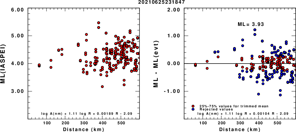
(a) ML computed using the IASPEI formula for Horizontal components; (b) ML residuals computed using a modified IASPEI formula that accounts for path specific attenuation; the values used for the trimmed mean are indicated. The ML relation used for each figure is given at the bottom of each plot.

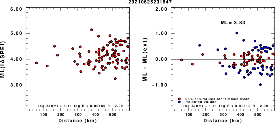
(a) ML computed using the IASPEI formula for Vertical components (research); (b) ML residuals computed using a modified IASPEI formula that accounts for path specific attenuation; the values used for the trimmed mean are indicated. The ML relation used for each figure is given at the bottom of each plot.

Context

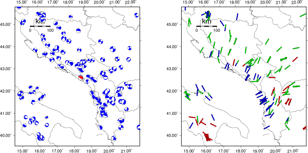
The next figure presents the focal mechanism for this earthquake (red) in the context of other events (blue) in the SLU Moment Tensor Catalog which are within ± 0.5 degrees of the new event. This comparison is shown in the left panel of the figure. The right panel shows the inferred direction of maximum compressive stress and the type of faulting (green is strike-slip, red is normal, blue is thrust; oblique is shown by a combination of colors).

Waveform Inversion

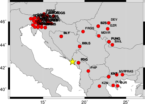
The focal mechanism was determined using broadband seismic waveforms. The location of the event and the and stations used for the waveform inversion are shown in the next figure.

Location of broadband stations used for waveform inversion

The program wvfgrd96 was used with good traces observed at short distance to determine the focal mechanism, depth and seismic moment. This technique requires a high quality signal and well determined velocity model for the Green functions. To the extent that these are the quality data, this type of mechanism should be preferred over the radiation pattern technique which requires the separate step of defining the pressure and tension quadrants and the correct strike.

The observed and predicted traces are filtered using the following gsac commands:

cut o DIST/3.3 -20 o DIST/3.3 +70
rtr
taper w 0.1
hp c 0.03 n 3 
lp c 0.08 n 3

The results of this grid search from 0.5 to 19 km depth are as follow:

           DEPTH  STK   DIP  RAKE   MW    FIT
WVFGRD96    1.0   105    45    90   3.88 0.2994
WVFGRD96    2.0   110    45   -85   4.00 0.3716
WVFGRD96    3.0   110    45   -85   4.05 0.3442
WVFGRD96    4.0   140    55   -40   3.98 0.2910
WVFGRD96    5.0   130    90   -65   4.01 0.3074
WVFGRD96    6.0   130    90    70   4.01 0.3563
WVFGRD96    7.0   130    90    70   4.02 0.3982
WVFGRD96    8.0   130    90    75   4.10 0.4275
WVFGRD96    9.0   125    90    75   4.12 0.4669
WVFGRD96   10.0   305    85   -75   4.13 0.4995
WVFGRD96   11.0   305    85   -75   4.15 0.5235
WVFGRD96   12.0   300    80   -70   4.16 0.5416
WVFGRD96   13.0   300    80   -70   4.17 0.5546
WVFGRD96   14.0   275    20    60   4.19 0.5665
WVFGRD96   15.0   275    20    60   4.20 0.5766
WVFGRD96   16.0   275    20    60   4.21 0.5828
WVFGRD96   17.0   275    20    60   4.22 0.5859
WVFGRD96   18.0   275    20    65   4.23 0.5878
WVFGRD96   19.0   275    20    65   4.24 0.5875
WVFGRD96   20.0   275    20    65   4.25 0.5851
WVFGRD96   21.0   270    20    60   4.27 0.5821
WVFGRD96   22.0   270    20    60   4.28 0.5760
WVFGRD96   23.0   270    20    60   4.29 0.5683
WVFGRD96   24.0   265    20    55   4.30 0.5590
WVFGRD96   25.0   265    20    55   4.30 0.5486
WVFGRD96   26.0   260    20    50   4.31 0.5368
WVFGRD96   27.0   260    20    50   4.32 0.5245
WVFGRD96   28.0   260    20    50   4.33 0.5109
WVFGRD96   29.0   255    20    45   4.33 0.4973

The best solution is

WVFGRD96   18.0   275    20    65   4.23 0.5878

The mechanism correspond to the best fit is

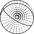
Figure 1. Waveform inversion focal mechanism

The best fit as a function of depth is given in the following figure:

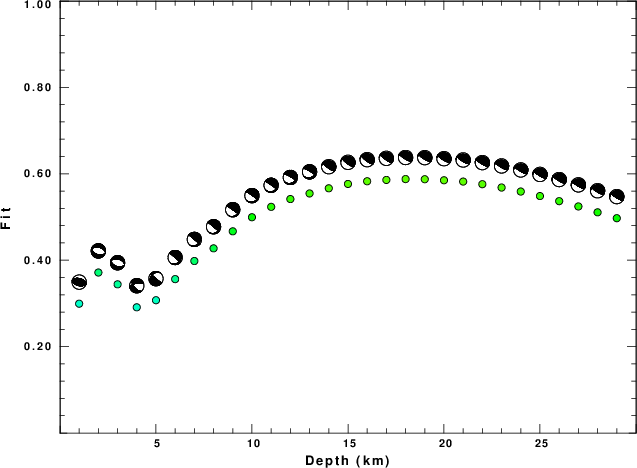
Figure 2. Depth sensitivity for waveform mechanism

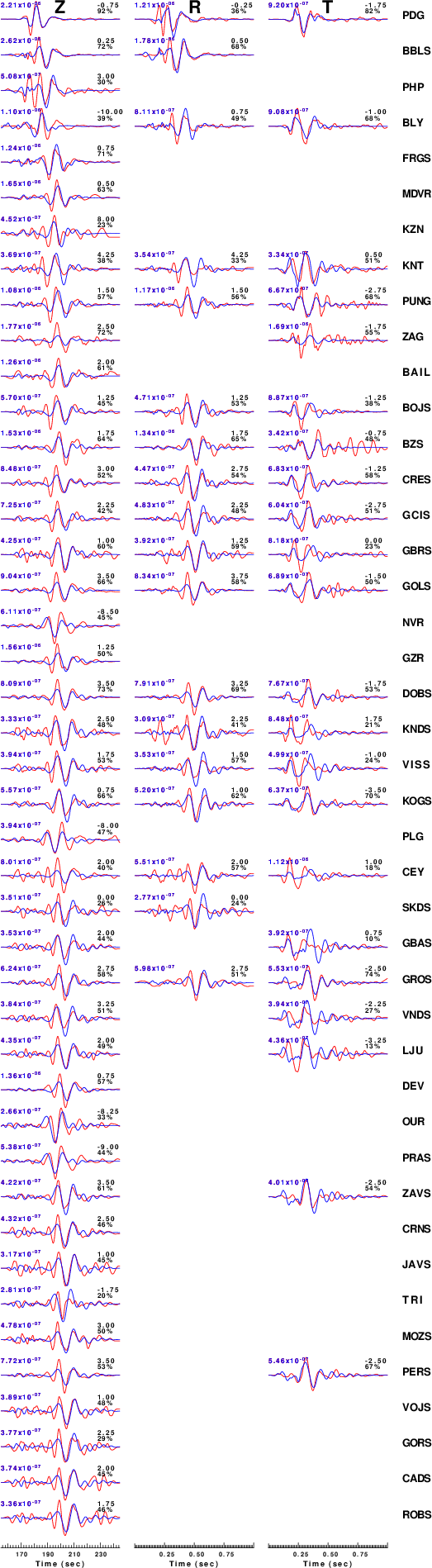
The comparison of the observed and predicted waveforms is given in the next figure. The red traces are the observed and the blue are the predicted. Each observed-predicted component is plotted to the same scale and peak amplitudes are indicated by the numbers to the left of each trace. A pair of numbers is given in black at the right of each predicted traces. The upper number it the time shift required for maximum correlation between the observed and predicted traces. This time shift is required because the synthetics are not computed at exactly the same distance as the observed and because the velocity model used in the predictions may not be perfect. A positive time shift indicates that the prediction is too fast and should be delayed to match the observed trace (shift to the right in this figure). A negative value indicates that the prediction is too slow. The lower number gives the percentage of variance reduction to characterize the individual goodness of fit (100% indicates a perfect fit).

The bandpass filter used in the processing and for the display was

cut o DIST/3.3 -20 o DIST/3.3 +70
rtr
taper w 0.1
hp c 0.03 n 3 
lp c 0.08 n 3

Figure 3. Waveform comparison for selected depth

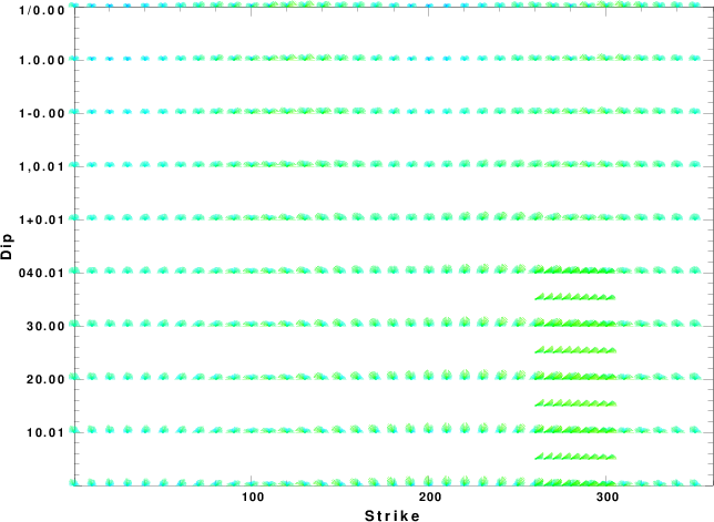
Focal mechanism sensitivity at the preferred depth. The red color indicates a very good fit to thewavefroms. Each solution is plotted as a vector at a given value of strike and dip with the angle of the vector representing the rake angle, measured, with respect to the upward vertical (N) in the figure.

A check on the assumed source location is possible by looking at the time shifts between the observed and predicted traces. The time shifts for waveform matching arise for several reasons:

The origin time and epicentral distance are incorrect
The velocity model used for the inversion is incorrect
The velocity model used to define the P-arrival time is not the same as the velocity model used for the waveform inversion (assuming that the initial trace alignment is based on the P arrival time)

Assuming only a mislocation, the time shifts are fit to a functional form:

 Time_shift = A + B cos Azimuth + C Sin Azimuth

The time shifts for this inversion lead to the next figure:

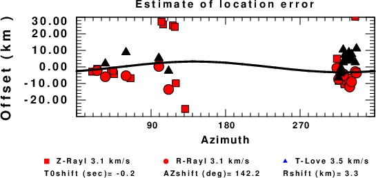
The derived shift in origin time and epicentral coordinates are given at the bottom of the figure.

Discussion

Acknowledgements

Thanks also to the many seismic network operators whose dedication make this effort possible: University of Nevada Reno, University of Alaska, University of Washington, Oregon State University, University of Utah, Montana Bureas of Mines, UC Berkely, Caltech, UC San Diego, Saint Louis University, University of Memphis, Lamont Doherty Earth Observatory, the Iris stations and the Transportable Array of EarthScope.

Velocity Model

The WUS.model used for the waveform synthetic seismograms and for the surface wave eigenfunctions and dispersion is as follows:

MODEL.01
Model after     8 iterations
ISOTROPIC
KGS
FLAT EARTH
1-D
CONSTANT VELOCITY
LINE08
LINE09
LINE10
LINE11
      H(KM)   VP(KM/S)   VS(KM/S) RHO(GM/CC)         QP         QS       ETAP       ETAS      FREFP      FREFS
     1.9000     3.4065     2.0089     2.2150  0.302E-02  0.679E-02   0.00       0.00       1.00       1.00    
     6.1000     5.5445     3.2953     2.6089  0.349E-02  0.784E-02   0.00       0.00       1.00       1.00    
    13.0000     6.2708     3.7396     2.7812  0.212E-02  0.476E-02   0.00       0.00       1.00       1.00    
    19.0000     6.4075     3.7680     2.8223  0.111E-02  0.249E-02   0.00       0.00       1.00       1.00    
     0.0000     7.9000     4.6200     3.2760  0.164E-10  0.370E-10   0.00       0.00       1.00       1.00

Quality Control

Here we tabulate the reasons for not using certain digital data sets

The following stations did not have a valid response files:

Last Changed Sat Jun 26 15:00:55 CDT 2021