Location

Location ANSS

2021/03/30 16:25:00 47.78 16.18 10.0 4.2 Austria

Focal Mechanism

USGS/SLU Moment Tensor Solution ENS 2021/03/30 16:25:00:7 47.78 16.18 10.0 4.2 Austria Stations used: BW.BGDS BW.BHG BW.ROTZ BW.RTBE BW.SCE CR.ZAG CZ.CHVC CZ.CKRC CZ.DPC CZ.KHC CZ.KRUC CZ.OSTC CZ.PRU CZ.STAC CZ.TREC CZ.UPC CZ.VRAC CZ.ZVC GR.FUR GR.GEC2 GR.GEC7 GR.GRC3 GR.WET HU.BUD HU.CSKK HU.EGYH HU.KOVH HU.MORH HU.MPLH HU.PSZ HU.SOP MN.TRI OE.ABTA OE.ARSA OE.BIOA OE.CONA OE.CSNA OE.KBA OE.LESA OE.MOA OE.MYKA OE.OBKA OE.SOKA OE.VIE OE.WATA OX.BAD OX.BOO OX.CIMO OX.CLUD OX.FUSE OX.MLN OX.PLRO OX.PRED OX.VARN SL.BOJS SL.CADS SL.CEY SL.CRES SL.CRNS SL.DOBS SL.GBAS SL.GBRS SL.GCIS SL.GOLS SL.GORS SL.GROS SL.JAVS SL.KNDS SL.KOGS SL.LJU SL.MOZS SL.PERS SL.ROBS SL.SKDS SL.VISS SL.VNDS SL.VOJS SL.ZAVS Filtering commands used: cut o DIST/3.3 -30 o DIST/3.3 +70 rtr taper w 0.1 hp c 0.03 n 3 lp c 0.06 n 3 Best Fitting Double Couple Mo = 1.17e+22 dyne-cm Mw = 3.98 Z = 13 km Plane Strike Dip Rake NP1 174 87 -125 NP2 80 35 -5 Principal Axes: Axis Value Plunge Azimuth T 1.17e+22 33 293 N 0.00e+00 35 176 P -1.17e+22 38 53 Moment Tensor: (dyne-cm) Component Value Mxx -1.36e+21 Mxy -6.47e+21 Mxz -1.32e+21 Myy 2.33e+21 Myz -9.50e+21 Mzz -9.62e+20 #####--------- #########------------- ############---------------- #############----------------- ###############------------------- ################----------- ------ ##### #########----------- P ------- ###### T ##########---------- -------- ###### ##########--------------------- ####################---------------------# ####################---------------------# ####################--------------------## #####################------------------### ####################-----------------### --##################---------------##### --#################-------------###### ----##############-----------####### ------############------########## ----------------############## ---------------############# -------------######### ---------##### Global CMT Convention Moment Tensor: R T P -9.62e+20 -1.32e+21 9.50e+21 -1.32e+21 -1.36e+21 6.47e+21 9.50e+21 6.47e+21 2.33e+21 Details of the solution is found at http://www.eas.slu.edu/eqc/eqc_mt/MECH.NA/20210330162500/index.html

Preferred Solution

The preferred solution from an analysis of the surface-wave spectral amplitude radiation pattern, waveform inversion and first motion observations is

      STK = 80
      DIP = 35
     RAKE = -5
       MW = 3.98
       HS = 13.0

The NDK file is 20210330162500.ndk The waveform inversion is preferred.

Moment Tensor Comparison

The following compares this source inversion to others

SLU

USGS/SLU Moment Tensor Solution ENS 2021/03/30 16:25:00:7 47.78 16.18 10.0 4.2 Austria Stations used: BW.BGDS BW.BHG BW.ROTZ BW.RTBE BW.SCE CR.ZAG CZ.CHVC CZ.CKRC CZ.DPC CZ.KHC CZ.KRUC CZ.OSTC CZ.PRU CZ.STAC CZ.TREC CZ.UPC CZ.VRAC CZ.ZVC GR.FUR GR.GEC2 GR.GEC7 GR.GRC3 GR.WET HU.BUD HU.CSKK HU.EGYH HU.KOVH HU.MORH HU.MPLH HU.PSZ HU.SOP MN.TRI OE.ABTA OE.ARSA OE.BIOA OE.CONA OE.CSNA OE.KBA OE.LESA OE.MOA OE.MYKA OE.OBKA OE.SOKA OE.VIE OE.WATA OX.BAD OX.BOO OX.CIMO OX.CLUD OX.FUSE OX.MLN OX.PLRO OX.PRED OX.VARN SL.BOJS SL.CADS SL.CEY SL.CRES SL.CRNS SL.DOBS SL.GBAS SL.GBRS SL.GCIS SL.GOLS SL.GORS SL.GROS SL.JAVS SL.KNDS SL.KOGS SL.LJU SL.MOZS SL.PERS SL.ROBS SL.SKDS SL.VISS SL.VNDS SL.VOJS SL.ZAVS Filtering commands used: cut o DIST/3.3 -30 o DIST/3.3 +70 rtr taper w 0.1 hp c 0.03 n 3 lp c 0.06 n 3 Best Fitting Double Couple Mo = 1.17e+22 dyne-cm Mw = 3.98 Z = 13 km Plane Strike Dip Rake NP1 174 87 -125 NP2 80 35 -5 Principal Axes: Axis Value Plunge Azimuth T 1.17e+22 33 293 N 0.00e+00 35 176 P -1.17e+22 38 53 Moment Tensor: (dyne-cm) Component Value Mxx -1.36e+21 Mxy -6.47e+21 Mxz -1.32e+21 Myy 2.33e+21 Myz -9.50e+21 Mzz -9.62e+20 #####--------- #########------------- ############---------------- #############----------------- ###############------------------- ################----------- ------ ##### #########----------- P ------- ###### T ##########---------- -------- ###### ##########--------------------- ####################---------------------# ####################---------------------# ####################--------------------## #####################------------------### ####################-----------------### --##################---------------##### --#################-------------###### ----##############-----------####### ------############------########## ----------------############## ---------------############# -------------######### ---------##### Global CMT Convention Moment Tensor: R T P -9.62e+20 -1.32e+21 9.50e+21 -1.32e+21 -1.36e+21 6.47e+21 9.50e+21 6.47e+21 2.33e+21 Details of the solution is found at http://www.eas.slu.edu/eqc/eqc_mt/MECH.NA/20210330162500/index.html

Magnitudes

ML Magnitude

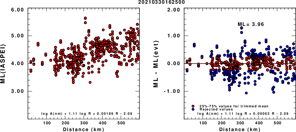
(a) ML computed using the IASPEI formula for Horizontal components; (b) ML residuals computed using a modified IASPEI formula that accounts for path specific attenuation; the values used for the trimmed mean are indicated. The ML relation used for each figure is given at the bottom of each plot.

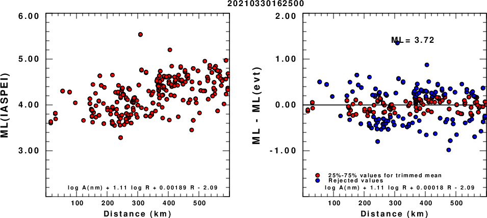
(a) ML computed using the IASPEI formula for Vertical components (research); (b) ML residuals computed using a modified IASPEI formula that accounts for path specific attenuation; the values used for the trimmed mean are indicated. The ML relation used for each figure is given at the bottom of each plot.

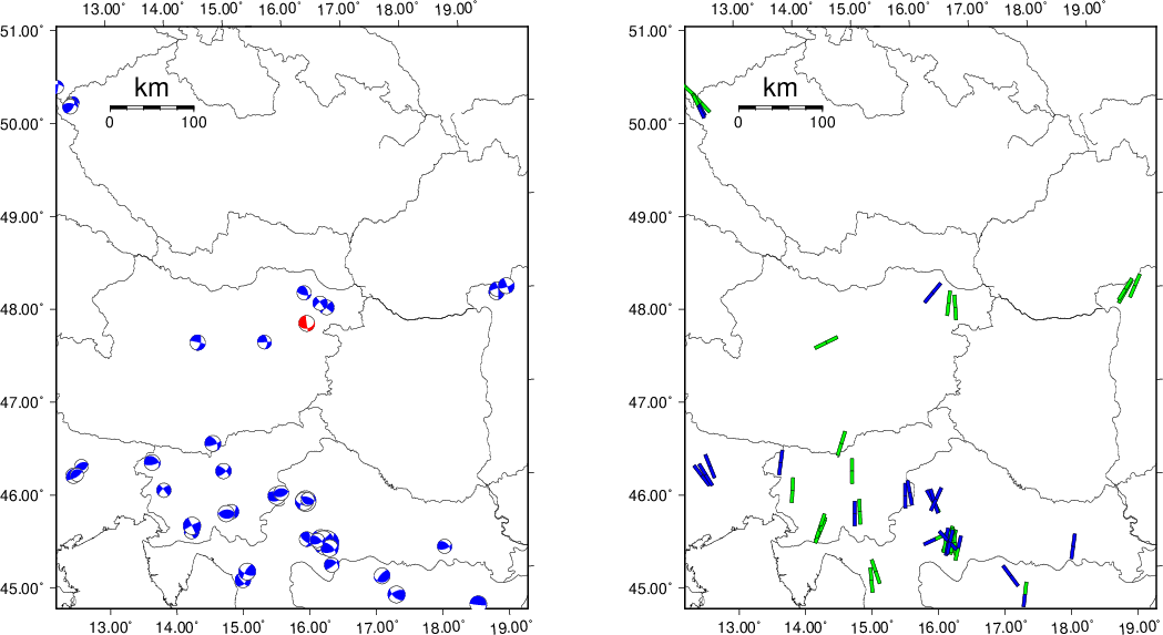
Context

The next figure presents the focal mechanism for this earthquake (red) in the context of other events (blue) in the SLU Moment Tensor Catalog which are within ± 0.5 degrees of the new event. This comparison is shown in the left panel of the figure. The right panel shows the inferred direction of maximum compressive stress and the type of faulting (green is strike-slip, red is normal, blue is thrust; oblique is shown by a combination of colors).

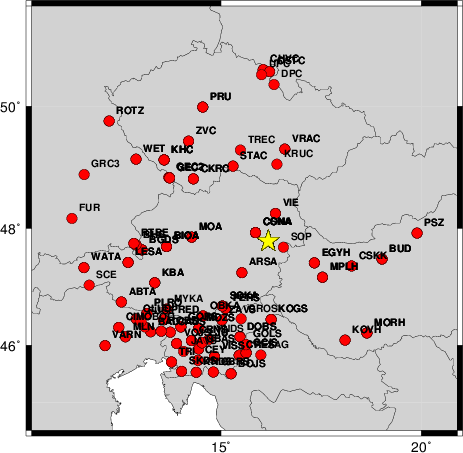
Waveform Inversion

The focal mechanism was determined using broadband seismic waveforms. The location of the event and the and stations used for the waveform inversion are shown in the next figure.

Location of broadband stations used for waveform inversion

The program wvfgrd96 was used with good traces observed at short distance to determine the focal mechanism, depth and seismic moment. This technique requires a high quality signal and well determined velocity model for the Green functions. To the extent that these are the quality data, this type of mechanism should be preferred over the radiation pattern technique which requires the separate step of defining the pressure and tension quadrants and the correct strike.

The observed and predicted traces are filtered using the following gsac commands:

cut o DIST/3.3 -30 o DIST/3.3 +70
rtr
taper w 0.1
hp c 0.03 n 3 
lp c 0.06 n 3

The results of this grid search from 0.5 to 19 km depth are as follow:

           DEPTH  STK   DIP  RAKE   MW    FIT
WVFGRD96    1.0    75    90    -5   3.62 0.3185
WVFGRD96    2.0   145    50    95   3.78 0.3612
WVFGRD96    3.0    75    85   -15   3.76 0.3613
WVFGRD96    4.0    90    30    15   3.87 0.3867
WVFGRD96    5.0    85    30    10   3.89 0.4352
WVFGRD96    6.0    85    30    10   3.89 0.4768
WVFGRD96    7.0    85    30     5   3.89 0.5082
WVFGRD96    8.0    85    25     5   3.96 0.5306
WVFGRD96    9.0    85    30     5   3.96 0.5539
WVFGRD96   10.0    85    30     5   3.97 0.5696
WVFGRD96   11.0    80    30    -5   3.97 0.5796
WVFGRD96   12.0    80    35    -5   3.98 0.5860
WVFGRD96   13.0    80    35    -5   3.98 0.5881
WVFGRD96   14.0    80    35    -5   3.99 0.5871
WVFGRD96   15.0    80    35    -5   3.99 0.5838
WVFGRD96   16.0    80    35    -5   4.00 0.5786
WVFGRD96   17.0    80    35    -5   4.00 0.5714
WVFGRD96   18.0    80    40    -5   4.01 0.5637
WVFGRD96   19.0    80    40    -5   4.01 0.5551
WVFGRD96   20.0    80    40    -5   4.02 0.5456
WVFGRD96   21.0    80    40    -5   4.03 0.5357
WVFGRD96   22.0    80    40    -5   4.03 0.5251
WVFGRD96   23.0    80    40   -10   4.04 0.5144
WVFGRD96   24.0    80    40   -10   4.04 0.5037
WVFGRD96   25.0    75    40   -15   4.05 0.4934
WVFGRD96   26.0    75    45   -15   4.06 0.4832
WVFGRD96   27.0    75    45   -15   4.06 0.4732
WVFGRD96   28.0    75    45   -20   4.07 0.4630
WVFGRD96   29.0    75    45   -20   4.07 0.4531

The best solution is

WVFGRD96   13.0    80    35    -5   3.98 0.5881

The mechanism correspond to the best fit is

Figure 1. Waveform inversion focal mechanism

The best fit as a function of depth is given in the following figure:

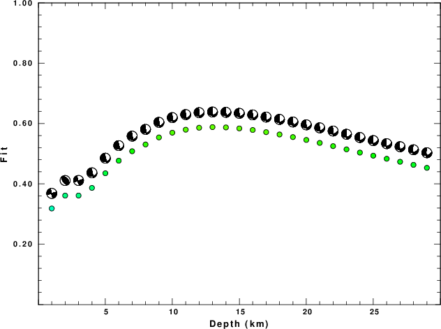
Figure 2. Depth sensitivity for waveform mechanism

The comparison of the observed and predicted waveforms is given in the next figure. The red traces are the observed and the blue are the predicted. Each observed-predicted component is plotted to the same scale and peak amplitudes are indicated by the numbers to the left of each trace. A pair of numbers is given in black at the right of each predicted traces. The upper number it the time shift required for maximum correlation between the observed and predicted traces. This time shift is required because the synthetics are not computed at exactly the same distance as the observed and because the velocity model used in the predictions may not be perfect. A positive time shift indicates that the prediction is too fast and should be delayed to match the observed trace (shift to the right in this figure). A negative value indicates that the prediction is too slow. The lower number gives the percentage of variance reduction to characterize the individual goodness of fit (100% indicates a perfect fit).

The bandpass filter used in the processing and for the display was

cut o DIST/3.3 -30 o DIST/3.3 +70
rtr
taper w 0.1
hp c 0.03 n 3 
lp c 0.06 n 3

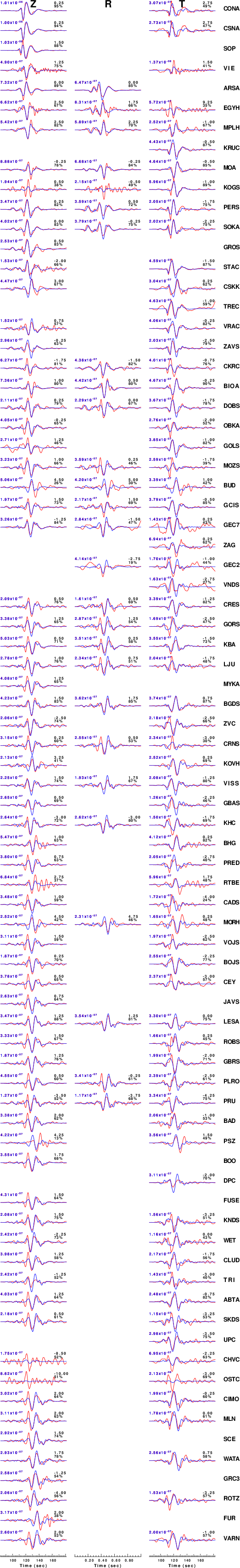
Figure 3. Waveform comparison for selected depth

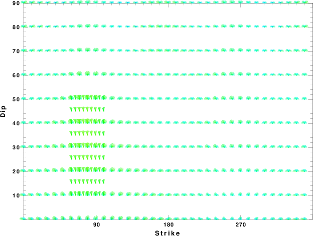
Focal mechanism sensitivity at the preferred depth. The red color indicates a very good fit to thewavefroms. Each solution is plotted as a vector at a given value of strike and dip with the angle of the vector representing the rake angle, measured, with respect to the upward vertical (N) in the figure.

A check on the assumed source location is possible by looking at the time shifts between the observed and predicted traces. The time shifts for waveform matching arise for several reasons:

The origin time and epicentral distance are incorrect
The velocity model used for the inversion is incorrect
The velocity model used to define the P-arrival time is not the same as the velocity model used for the waveform inversion (assuming that the initial trace alignment is based on the P arrival time)

Assuming only a mislocation, the time shifts are fit to a functional form:

 Time_shift = A + B cos Azimuth + C Sin Azimuth

The time shifts for this inversion lead to the next figure:

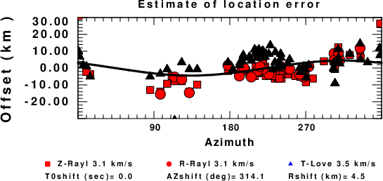
The derived shift in origin time and epicentral coordinates are given at the bottom of the figure.

Discussion

Acknowledgements

Thanks also to the many seismic network operators whose dedication make this effort possible: University of Nevada Reno, University of Alaska, University of Washington, Oregon State University, University of Utah, Montana Bureas of Mines, UC Berkely, Caltech, UC San Diego, Saint Louis University, University of Memphis, Lamont Doherty Earth Observatory, the Iris stations and the Transportable Array of EarthScope.

Velocity Model

The WUS.model used for the waveform synthetic seismograms and for the surface wave eigenfunctions and dispersion is as follows:

MODEL.01
Model after     8 iterations
ISOTROPIC
KGS
FLAT EARTH
1-D
CONSTANT VELOCITY
LINE08
LINE09
LINE10
LINE11
      H(KM)   VP(KM/S)   VS(KM/S) RHO(GM/CC)         QP         QS       ETAP       ETAS      FREFP      FREFS
     1.9000     3.4065     2.0089     2.2150  0.302E-02  0.679E-02   0.00       0.00       1.00       1.00    
     6.1000     5.5445     3.2953     2.6089  0.349E-02  0.784E-02   0.00       0.00       1.00       1.00    
    13.0000     6.2708     3.7396     2.7812  0.212E-02  0.476E-02   0.00       0.00       1.00       1.00    
    19.0000     6.4075     3.7680     2.8223  0.111E-02  0.249E-02   0.00       0.00       1.00       1.00    
     0.0000     7.9000     4.6200     3.2760  0.164E-10  0.370E-10   0.00       0.00       1.00       1.00

Quality Control

Here we tabulate the reasons for not using certain digital data sets

The following stations did not have a valid response files:

Last Changed Thu Apr 1 10:03:02 CDT 2021