Location
Location ANSS
2021/01/12 22:09:55 38.39 22.05 4.0 4.9 Greece
Focal Mechanism
 USGS/SLU Moment Tensor Solution
 ENS  2021/01/12 22:09:55:5  38.39   22.05   4.0 4.9 Greece

 Stations used:
   HL.ATH HL.DION HL.EVR HL.ITM HL.JAN HL.KYMI HL.LKR HL.NEO
   HL.NVR HL.PTL HL.RLS HL.TETR HL.VLI HL.VLS HL.VLY HT.AGG
   HT.AOS2 HT.EVGI HT.GRG HT.IGT HT.KPRO HT.LKD2 HT.OUR
   HT.PAIG HT.PSDA HT.RTZL HT.SRS HT.THAS MN.KEK MN.KLV
   SJ.BBLS

 Filtering commands used:
   cut o DIST/3.3 -30 o DIST/3.3 +70
   rtr
   taper w 0.1
   hp c 0.03 n 3
   lp c 0.08 n 3

 Best Fitting Double Couple
  Mo = 3.24e+23 dyne-cm
  Mw = 4.94
  Z  = 11 km
  Plane   Strike  Dip  Rake
   NP1      310    80   -35
   NP2       47    56   -168
  Principal Axes:
   Axis    Value   Plunge  Azimuth
    T   3.24e+23     16       3
    N   0.00e+00     54     116
    P  -3.24e+23     31     263

 Moment Tensor: (dyne-cm)
    Component   Value
       Mxx     2.94e+23
       Mxy    -1.41e+22
       Mxz     1.04e+23
       Myy    -2.31e+23
       Myz     1.47e+23
       Mzz    -6.35e+22


                     ######   #####
                 ########## T #########
              #############   ############
             ##############################
           ----############################--
          --------#########################---
         ------------######################----
        ----------------##################------
        ------------------################------
       ----------------------############--------
       -----   ----------------#########---------
       ----- P ------------------######----------
       -----   --------------------##------------
        ----------------------------#-----------
        --------------------------#####---------
         -----------------------########-------
          -------------------#############----
           ---------------#################--
             --------######################
              ############################
                 ######################
                     ##############


 Global CMT Convention Moment Tensor:
      R          T          P
 -6.35e+22   1.04e+23  -1.47e+23
  1.04e+23   2.94e+23   1.41e+22
 -1.47e+23   1.41e+22  -2.31e+23


Details of the solution is found at

http://www.eas.slu.edu/eqc/eqc_mt/MECH.NA/20210112220955/index.html
|
Preferred Solution
The preferred solution from an analysis of the surface-wave spectral amplitude radiation pattern, waveform inversion and first motion observations is
      STK = 310
      DIP = 80
     RAKE = -35
       MW = 4.94
       HS = 11.0
The NDK file is 20210112220955.ndk
The waveform inversion is preferred.
Moment Tensor Comparison
The following compares this source inversion to others
| SLU |
OTHER |
 USGS/SLU Moment Tensor Solution
 ENS  2021/01/12 22:09:55:5  38.39   22.05   4.0 4.9 Greece

 Stations used:
   HL.ATH HL.DION HL.EVR HL.ITM HL.JAN HL.KYMI HL.LKR HL.NEO
   HL.NVR HL.PTL HL.RLS HL.TETR HL.VLI HL.VLS HL.VLY HT.AGG
   HT.AOS2 HT.EVGI HT.GRG HT.IGT HT.KPRO HT.LKD2 HT.OUR
   HT.PAIG HT.PSDA HT.RTZL HT.SRS HT.THAS MN.KEK MN.KLV
   SJ.BBLS

 Filtering commands used:
   cut o DIST/3.3 -30 o DIST/3.3 +70
   rtr
   taper w 0.1
   hp c 0.03 n 3
   lp c 0.08 n 3

 Best Fitting Double Couple
  Mo = 3.24e+23 dyne-cm
  Mw = 4.94
  Z  = 11 km
  Plane   Strike  Dip  Rake
   NP1      310    80   -35
   NP2       47    56   -168
  Principal Axes:
   Axis    Value   Plunge  Azimuth
    T   3.24e+23     16       3
    N   0.00e+00     54     116
    P  -3.24e+23     31     263

 Moment Tensor: (dyne-cm)
    Component   Value
       Mxx     2.94e+23
       Mxy    -1.41e+22
       Mxz     1.04e+23
       Myy    -2.31e+23
       Myz     1.47e+23
       Mzz    -6.35e+22


                     ######   #####
                 ########## T #########
              #############   ############
             ##############################
           ----############################--
          --------#########################---
         ------------######################----
        ----------------##################------
        ------------------################------
       ----------------------############--------
       -----   ----------------#########---------
       ----- P ------------------######----------
       -----   --------------------##------------
        ----------------------------#-----------
        --------------------------#####---------
         -----------------------########-------
          -------------------#############----
           ---------------#################--
             --------######################
              ############################
                 ######################
                     ##############


 Global CMT Convention Moment Tensor:
      R          T          P
 -6.35e+22   1.04e+23  -1.47e+23
  1.04e+23   2.94e+23   1.41e+22
 -1.47e+23   1.41e+22  -2.31e+23


Details of the solution is found at

http://www.eas.slu.edu/eqc/eqc_mt/MECH.NA/20210112220955/index.html
|
NOA - Athens
result_complete.pdf
|
Magnitudes
ML Magnitude
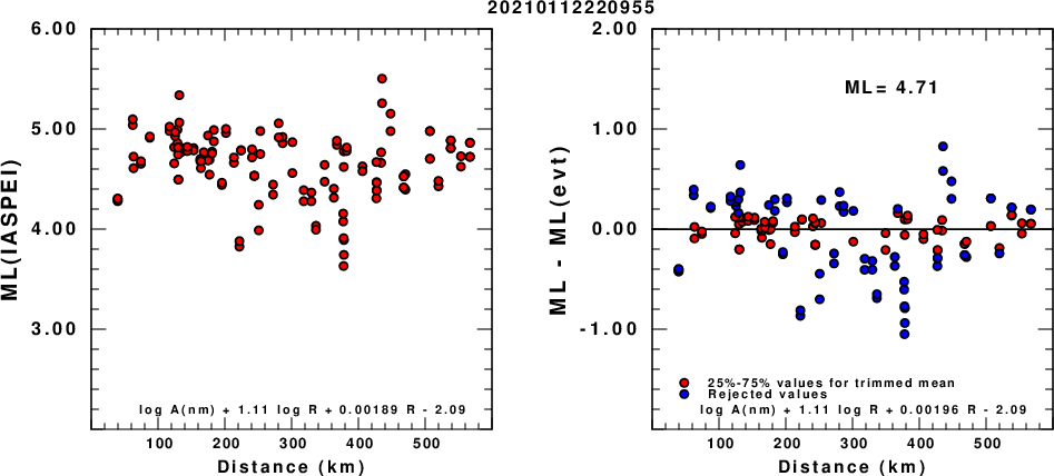
(a) ML computed using the IASPEI formula for Horizontal components; (b) ML residuals computed using a modified IASPEI formula that accounts for path specific attenuation; the values used for the trimmed mean are indicated. The ML relation used for each figure is given at the bottom of each plot.
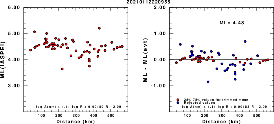
(a) ML computed using the IASPEI formula for Vertical components (research); (b) ML residuals computed using a modified IASPEI formula that accounts for path specific attenuation; the values used for the trimmed mean are indicated. The ML relation used for each figure is given at the bottom of each plot.
Context
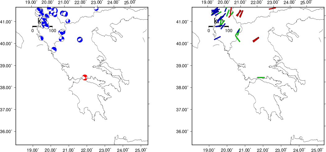
The next figure presents the focal mechanism for this earthquake (red) in the context of other events (blue) in the SLU Moment Tensor Catalog which are within ± 0.5 degrees of the new event. This comparison is shown in the left panel of the figure. The right panel shows the inferred direction of maximum compressive stress and the type of faulting (green is strike-slip, red is normal, blue is thrust; oblique is shown by a combination of colors).
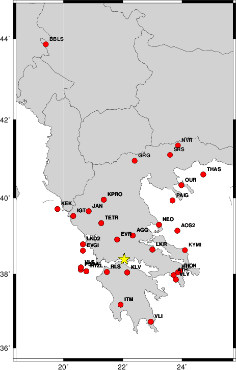
Waveform Inversion
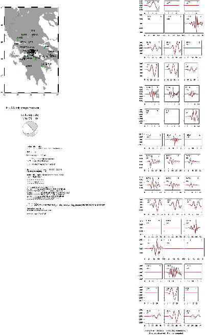
The focal mechanism was determined using broadband seismic waveforms. The location of the event and the
and stations used for the waveform inversion are shown in the next figure.
|
|
Location of broadband stations used for waveform inversion
|
The program wvfgrd96 was used with good traces observed at short distance to determine the focal mechanism, depth and seismic moment. This technique requires a high quality signal and well determined velocity model for the Green functions. To the extent that these are the quality data, this type of mechanism should be preferred over the radiation pattern technique which requires the separate step of defining the pressure and tension quadrants and the correct strike.
The observed and predicted traces are filtered using the following gsac commands:
cut o DIST/3.3 -30 o DIST/3.3 +70
rtr
taper w 0.1
hp c 0.03 n 3
lp c 0.08 n 3
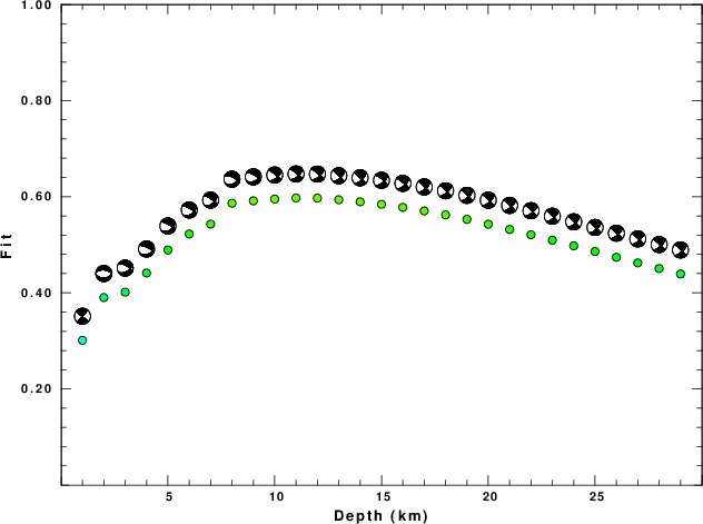
The results of this grid search from 0.5 to 19 km depth are as follow:
           DEPTH  STK   DIP  RAKE   MW    FIT
WVFGRD96    1.0   130    85     0   4.51 0.3013
WVFGRD96    2.0   275    50   -85   4.75 0.3902
WVFGRD96    3.0   300    60   -50   4.76 0.4015
WVFGRD96    4.0   295    70   -65   4.82 0.4413
WVFGRD96    5.0   300    70   -55   4.82 0.4892
WVFGRD96    6.0   300    70   -55   4.83 0.5224
WVFGRD96    7.0   305    75   -45   4.84 0.5430
WVFGRD96    8.0   295    65   -60   4.93 0.5864
WVFGRD96    9.0   300    65   -55   4.93 0.5914
WVFGRD96   10.0   310    80   -40   4.92 0.5952
WVFGRD96   11.0   310    80   -35   4.94 0.5974
WVFGRD96   12.0   310    80   -35   4.95 0.5971
WVFGRD96   13.0   315    90   -30   4.96 0.5937
WVFGRD96   14.0   315    90   -30   4.97 0.5894
WVFGRD96   15.0   310    75   -30   4.98 0.5842
WVFGRD96   16.0   310    80   -30   4.99 0.5778
WVFGRD96   17.0   315    85   -25   5.00 0.5704
WVFGRD96   18.0   315    85   -25   5.01 0.5623
WVFGRD96   19.0   315    85   -25   5.02 0.5529
WVFGRD96   20.0   315    85   -25   5.02 0.5428
WVFGRD96   21.0   315    85   -25   5.03 0.5319
WVFGRD96   22.0   315    85   -25   5.04 0.5209
WVFGRD96   23.0   315    85   -25   5.04 0.5095
WVFGRD96   24.0   315    85   -25   5.05 0.4978
WVFGRD96   25.0   315    85   -25   5.06 0.4860
WVFGRD96   26.0   315    85   -25   5.06 0.4741
WVFGRD96   27.0   315    85   -25   5.07 0.4623
WVFGRD96   28.0   315    85   -25   5.07 0.4505
WVFGRD96   29.0   315    85   -25   5.08 0.4392
The best solution is
WVFGRD96 11.0 310 80 -35 4.94 0.5974
The mechanism correspond to the best fit is
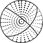
|
|
Figure 1. Waveform inversion focal mechanism
|
The best fit as a function of depth is given in the following figure:
|
|
Figure 2. Depth sensitivity for waveform mechanism
|
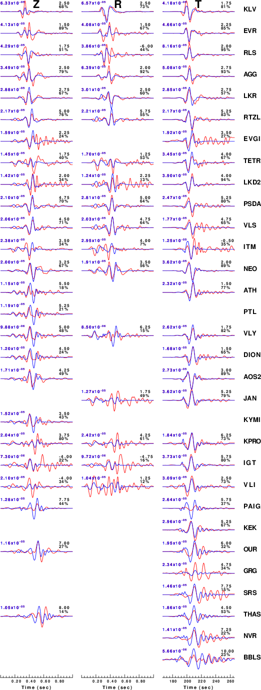
The comparison of the observed and predicted waveforms is given in the next figure. The red traces are the observed and the blue are the predicted.
Each observed-predicted component is plotted to the same scale and peak amplitudes are indicated by the numbers to the left of each trace. A pair of numbers is given in black at the right of each predicted traces. The upper number it the time shift required for maximum correlation between the observed and predicted traces. This time shift is required because the synthetics are not computed at exactly the same distance as the observed and because the velocity model used in the predictions may not be perfect.
A positive time shift indicates that the prediction is too fast and should be delayed to match the observed trace (shift to the right in this figure). A negative value indicates that the prediction is too slow. The lower number gives the percentage of variance reduction to characterize the individual goodness of fit (100% indicates a perfect fit).
The bandpass filter used in the processing and for the display was
cut o DIST/3.3 -30 o DIST/3.3 +70
rtr
taper w 0.1
hp c 0.03 n 3
lp c 0.08 n 3
|
|
Figure 3. Waveform comparison for selected depth
|
|
|
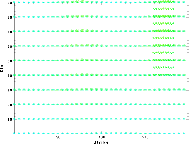
Focal mechanism sensitivity at the preferred depth. The red color indicates a very good fit to thewavefroms.
Each solution is plotted as a vector at a given value of strike and dip with the angle of the vector representing the rake angle, measured, with respect to the upward vertical (N) in the figure.
|
A check on the assumed source location is possible by looking at the time shifts between the observed and predicted traces. The time shifts for waveform matching arise for several reasons:
- The origin time and epicentral distance are incorrect
- The velocity model used for the inversion is incorrect
- The velocity model used to define the P-arrival time is not the
same as the velocity model used for the waveform inversion
(assuming that the initial trace alignment is based on the
P arrival time)
Assuming only a mislocation, the time shifts are fit to a functional form:
Time_shift = A + B cos Azimuth + C Sin Azimuth
The time shifts for this inversion lead to the next figure:
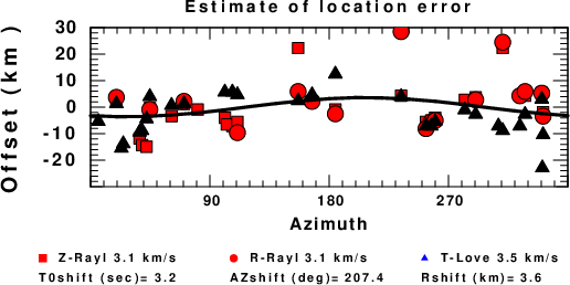
The derived shift in origin time and epicentral coordinates are given at the bottom of the figure.
Discussion
Acknowledgements
Thanks also to the many seismic network operators whose dedication make this effort possible: University of Nevada Reno, University of Alaska, University of Washington, Oregon State University, University of Utah, Montana Bureas of Mines, UC Berkely, Caltech, UC San Diego, Saint Louis University, University of Memphis, Lamont Doherty Earth Observatory, the Iris stations and the Transportable Array of EarthScope.
Velocity Model
The WUS.model used for the waveform synthetic seismograms and for the surface wave eigenfunctions and dispersion is as follows:
MODEL.01
Model after     8 iterations
ISOTROPIC
KGS
FLAT EARTH
1-D
CONSTANT VELOCITY
LINE08
LINE09
LINE10
LINE11
      H(KM)   VP(KM/S)   VS(KM/S) RHO(GM/CC)         QP         QS       ETAP       ETAS      FREFP      FREFS
     1.9000     3.4065     2.0089     2.2150  0.302E-02  0.679E-02   0.00       0.00       1.00       1.00
     6.1000     5.5445     3.2953     2.6089  0.349E-02  0.784E-02   0.00       0.00       1.00       1.00
    13.0000     6.2708     3.7396     2.7812  0.212E-02  0.476E-02   0.00       0.00       1.00       1.00
    19.0000     6.4075     3.7680     2.8223  0.111E-02  0.249E-02   0.00       0.00       1.00       1.00
     0.0000     7.9000     4.6200     3.2760  0.164E-10  0.370E-10   0.00       0.00       1.00       1.00
Quality Control
Here we tabulate the reasons for not using certain digital data sets
The following stations did not have a valid response files:
Last Changed Tue Jan 12 18:06:31 CST 2021