Location
Location ANSS
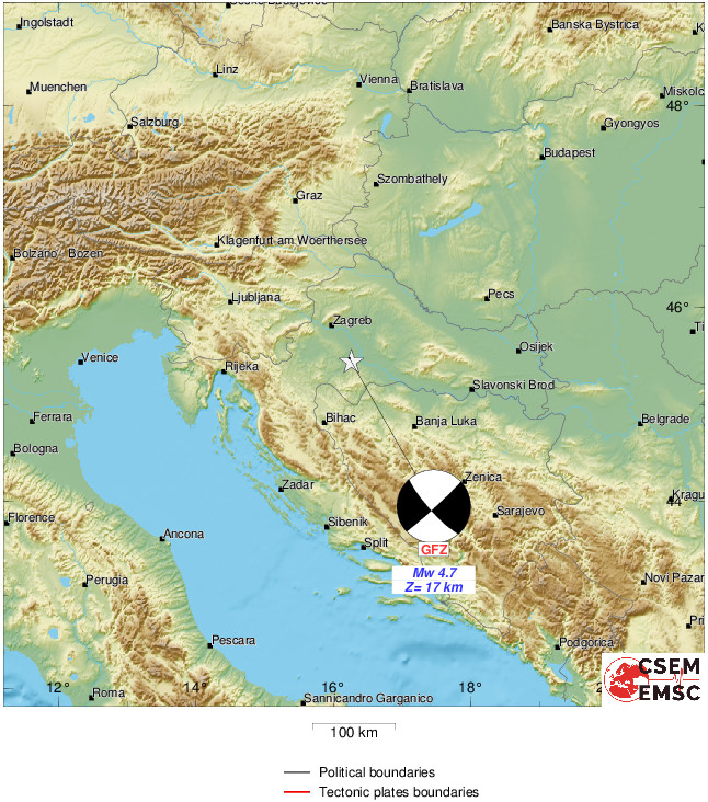
2021/01/06 17:01:43 45.44 16.26 10.0 5.0 Croatia
Focal Mechanism
 USGS/SLU Moment Tensor Solution
 ENS  2021/01/06 17:01:43:1  45.44   16.26  10.0 5.0 Croatia

 Stations used:
   AC.BCI BW.ALFT BW.BGDS BW.BIB BW.FFB1 BW.GELB BW.GRMB
   BW.KW1 BW.MGS02 BW.MGS03 BW.MGS05 BW.PART BW.RNHA BW.RNON
   BW.ROTZ BW.SCE BW.ZUGS CH.BERNI CH.DAVOX CH.FUORN CH.LIENZ
   CH.LLS CH.PLONS CH.ROMAN CH.SGT05 CH.VDR CR.ZAG GE.MATE
   GR.FUR GR.GEC7 GR.GRA4 GR.GRB4 GR.GRC1 GR.GRC2 GR.GRC3
   GR.GRC4 GR.UBR GR.WET HU.AMBH HU.BEHE HU.BSZH HU.BUD
   HU.CSKK HU.EGYH HU.KOVH HU.MORH HU.PSZ HU.SOP HU.TIH MN.BLY
   MN.PDG MN.TRI MN.TUE OE.ABTA OE.ARSA OE.BIOA OE.CONA
   OE.CSNA OE.DAVA OE.FETA OE.KBA OE.LESA OE.MOA OE.MOTA
   OE.MYKA OE.OBKA OE.RETA OE.RONA OE.SOKA OE.SQTA OE.VIE
   OE.WATA OX.ACOM OX.AGOR OX.BAD OX.BOO OX.CAE OX.CIMO
   OX.CLUD OX.DRE OX.MLN OX.MPRI OX.SABO RO.BZS RO.PUNG
   SL.BOJS SL.CADS SL.CEY SL.CRES SL.CRNS SL.DOBS SL.GBAS
   SL.GBRS SL.GCIS SL.GOLS SL.GORS SL.GROS SL.JAVS SL.KNDS
   SL.LJU SL.MOZS SL.PDKS SL.PERS SL.ROBS SL.SKDS SL.VISS
   SL.VNDS SL.ZAVS

 Filtering commands used:
   cut o DIST/3.3 -40 o DIST/3.3 +50
   rtr
   taper w 0.1
   hp c 0.03 n 3
   lp c 0.06 n 3

 Best Fitting Double Couple
  Mo = 1.62e+23 dyne-cm
  Mw = 4.74
  Z  = 13 km
  Plane   Strike  Dip  Rake
   NP1       50    90    10
   NP2      320    80   180
  Principal Axes:
   Axis    Value   Plunge  Azimuth
    T   1.62e+23      7     275
    N   0.00e+00     80      50
    P  -1.62e+23      7     185

 Moment Tensor: (dyne-cm)
    Component   Value
       Mxx    -1.57e+23
       Mxy    -2.77e+22
       Mxz     2.16e+22
       Myy     1.57e+23
       Myz    -1.81e+22
       Mzz    -2.46e+15


                     --------------
                 ----------------------
              #---------------------------
             #####-------------------------
           #########----------------------###
          ############------------------######
         ###############--------------#########
        ##################----------############
        ###################-------##############
          ###################--##################
        T ###################--##################
          #################-----#################
       ##################--------################
        ##############-------------#############
        ############----------------############
         #########-------------------##########
          ######-----------------------#######
           ###--------------------------#####
             ---------------------------###
              ---------------------------#
                 --------   -----------
                     ---- P -------


 Global CMT Convention Moment Tensor:
      R          T          P
 -2.46e+15   2.16e+22   1.81e+22
  2.16e+22  -1.57e+23   2.77e+22
  1.81e+22   2.77e+22   1.57e+23


Details of the solution is found at

http://www.eas.slu.edu/eqc/eqc_mt/MECH.NA/20210106170143/index.html
|
Preferred Solution
The preferred solution from an analysis of the surface-wave spectral amplitude radiation pattern, waveform inversion and first motion observations is
      STK = 50
      DIP = 90
     RAKE = 10
       MW = 4.74
       HS = 13.0
The NDK file is 20210106170143.ndk
The waveform inversion is preferred.
Moment Tensor Comparison
The following compares this source inversion to others
| SLU |
OTHER |
 USGS/SLU Moment Tensor Solution
 ENS  2021/01/06 17:01:43:1  45.44   16.26  10.0 5.0 Croatia

 Stations used:
   AC.BCI BW.ALFT BW.BGDS BW.BIB BW.FFB1 BW.GELB BW.GRMB
   BW.KW1 BW.MGS02 BW.MGS03 BW.MGS05 BW.PART BW.RNHA BW.RNON
   BW.ROTZ BW.SCE BW.ZUGS CH.BERNI CH.DAVOX CH.FUORN CH.LIENZ
   CH.LLS CH.PLONS CH.ROMAN CH.SGT05 CH.VDR CR.ZAG GE.MATE
   GR.FUR GR.GEC7 GR.GRA4 GR.GRB4 GR.GRC1 GR.GRC2 GR.GRC3
   GR.GRC4 GR.UBR GR.WET HU.AMBH HU.BEHE HU.BSZH HU.BUD
   HU.CSKK HU.EGYH HU.KOVH HU.MORH HU.PSZ HU.SOP HU.TIH MN.BLY
   MN.PDG MN.TRI MN.TUE OE.ABTA OE.ARSA OE.BIOA OE.CONA
   OE.CSNA OE.DAVA OE.FETA OE.KBA OE.LESA OE.MOA OE.MOTA
   OE.MYKA OE.OBKA OE.RETA OE.RONA OE.SOKA OE.SQTA OE.VIE
   OE.WATA OX.ACOM OX.AGOR OX.BAD OX.BOO OX.CAE OX.CIMO
   OX.CLUD OX.DRE OX.MLN OX.MPRI OX.SABO RO.BZS RO.PUNG
   SL.BOJS SL.CADS SL.CEY SL.CRES SL.CRNS SL.DOBS SL.GBAS
   SL.GBRS SL.GCIS SL.GOLS SL.GORS SL.GROS SL.JAVS SL.KNDS
   SL.LJU SL.MOZS SL.PDKS SL.PERS SL.ROBS SL.SKDS SL.VISS
   SL.VNDS SL.ZAVS

 Filtering commands used:
   cut o DIST/3.3 -40 o DIST/3.3 +50
   rtr
   taper w 0.1
   hp c 0.03 n 3
   lp c 0.06 n 3

 Best Fitting Double Couple
  Mo = 1.62e+23 dyne-cm
  Mw = 4.74
  Z  = 13 km
  Plane   Strike  Dip  Rake
   NP1       50    90    10
   NP2      320    80   180
  Principal Axes:
   Axis    Value   Plunge  Azimuth
    T   1.62e+23      7     275
    N   0.00e+00     80      50
    P  -1.62e+23      7     185

 Moment Tensor: (dyne-cm)
    Component   Value
       Mxx    -1.57e+23
       Mxy    -2.77e+22
       Mxz     2.16e+22
       Myy     1.57e+23
       Myz    -1.81e+22
       Mzz    -2.46e+15


                     --------------
                 ----------------------
              #---------------------------
             #####-------------------------
           #########----------------------###
          ############------------------######
         ###############--------------#########
        ##################----------############
        ###################-------##############
          ###################--##################
        T ###################--##################
          #################-----#################
       ##################--------################
        ##############-------------#############
        ############----------------############
         #########-------------------##########
          ######-----------------------#######
           ###--------------------------#####
             ---------------------------###
              ---------------------------#
                 --------   -----------
                     ---- P -------


 Global CMT Convention Moment Tensor:
      R          T          P
 -2.46e+15   2.16e+22   1.81e+22
  2.16e+22  -1.57e+23   2.77e+22
  1.81e+22   2.77e+22   1.57e+23


Details of the solution is found at

http://www.eas.slu.edu/eqc/eqc_mt/MECH.NA/20210106170143/index.html
|
 https://www.croatiaweek.com/magnitude-5-0-earthquake-hits-central-croatia/


http://geofon.gfz-potsdam.de/eqinfo/event.php?id=gfz2021aklf
Time
2021-01-06 17:01:44
Magnitude
4.7
Latitude
45.48°N
Longitude
16.23°E
Depth
17 km
Nodal planes
Strike	Dip	Rake
138°	80°	-177°
48°	87°	-9°
https://static2.emsc.eu/Images/EVID/93/936/936384/936384.MT.jpg
|
Magnitudes
ML Magnitude
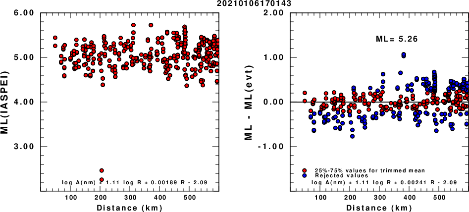
(a) ML computed using the IASPEI formula for Horizontal components; (b) ML residuals computed using a modified IASPEI formula that accounts for path specific attenuation; the values used for the trimmed mean are indicated. The ML relation used for each figure is given at the bottom of each plot.
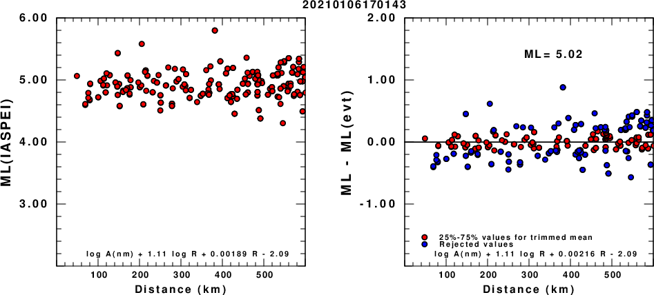
(a) ML computed using the IASPEI formula for Vertical components (research); (b) ML residuals computed using a modified IASPEI formula that accounts for path specific attenuation; the values used for the trimmed mean are indicated. The ML relation used for each figure is given at the bottom of each plot.
Context
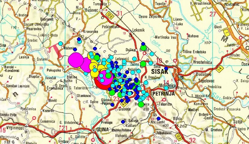
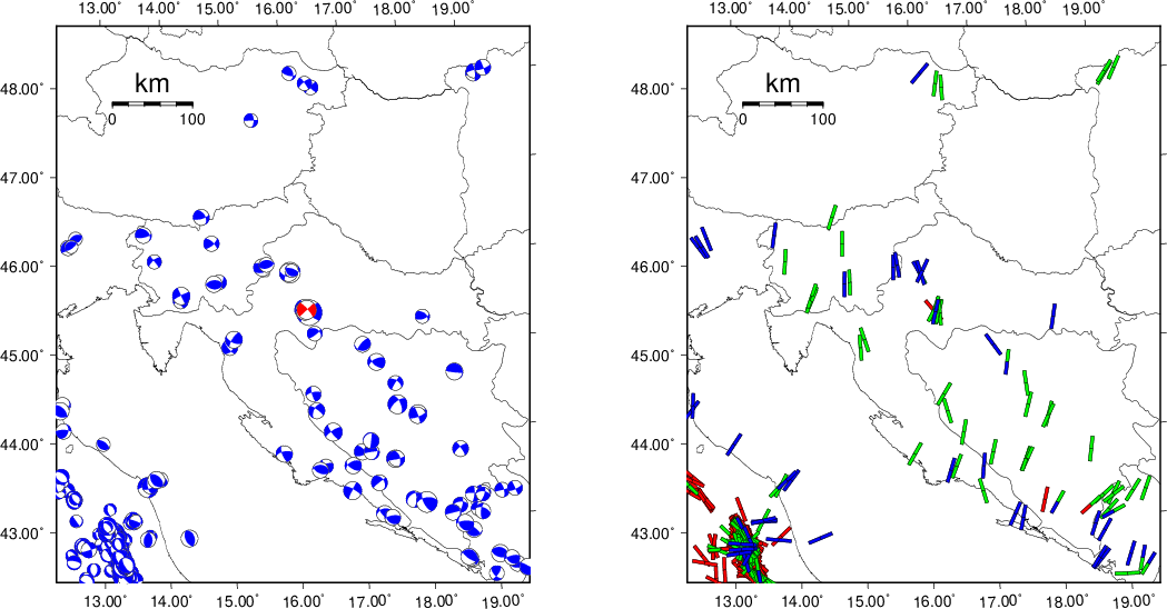
The next figure presents the focal mechanism for this earthquake (red) in the context of other events (blue) in the SLU Moment Tensor Catalog which are within ± 0.5 degrees of the new event. This comparison is shown in the left panel of the figure. The right panel shows the inferred direction of maximum compressive stress and the type of faulting (green is strike-slip, red is normal, blue is thrust; oblique is shown by a combination of colors).
Waveform Inversion
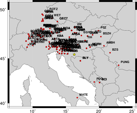
The focal mechanism was determined using broadband seismic waveforms. The location of the event and the
and stations used for the waveform inversion are shown in the next figure.
|
|
Location of broadband stations used for waveform inversion
|
The program wvfgrd96 was used with good traces observed at short distance to determine the focal mechanism, depth and seismic moment. This technique requires a high quality signal and well determined velocity model for the Green functions. To the extent that these are the quality data, this type of mechanism should be preferred over the radiation pattern technique which requires the separate step of defining the pressure and tension quadrants and the correct strike.
The observed and predicted traces are filtered using the following gsac commands:
cut o DIST/3.3 -40 o DIST/3.3 +50
rtr
taper w 0.1
hp c 0.03 n 3
lp c 0.06 n 3
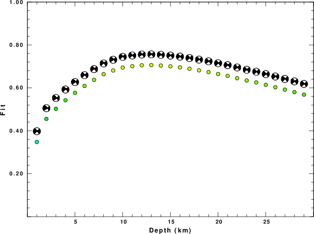
The results of this grid search from 0.5 to 19 km depth are as follow:
           DEPTH  STK   DIP  RAKE   MW    FIT
WVFGRD96    1.0    50    85    10   4.35 0.3478
WVFGRD96    2.0    55    75    25   4.49 0.4552
WVFGRD96    3.0    55    75    20   4.53 0.5026
WVFGRD96    4.0    50    90    20   4.55 0.5423
WVFGRD96    5.0   230    90   -20   4.58 0.5769
WVFGRD96    6.0    50    90    15   4.60 0.6089
WVFGRD96    7.0   230    85   -15   4.63 0.6373
WVFGRD96    8.0   230    85   -15   4.66 0.6637
WVFGRD96    9.0    50    90    15   4.68 0.6809
WVFGRD96   10.0   230    85   -15   4.70 0.6945
WVFGRD96   11.0    50    90    10   4.71 0.7007
WVFGRD96   12.0    50    90    10   4.72 0.7053
WVFGRD96   13.0    50    90    10   4.74 0.7060
WVFGRD96   14.0   230    90   -10   4.75 0.7039
WVFGRD96   15.0    50    90    10   4.76 0.7003
WVFGRD96   16.0   230    90   -10   4.76 0.6955
WVFGRD96   17.0   230    90   -10   4.77 0.6890
WVFGRD96   18.0   230    90   -10   4.78 0.6816
WVFGRD96   19.0    50    90    10   4.79 0.6736
WVFGRD96   20.0    50    85    10   4.80 0.6648
WVFGRD96   21.0    50    85    10   4.80 0.6558
WVFGRD96   22.0   230    90   -10   4.81 0.6450
WVFGRD96   23.0   230    90   -10   4.81 0.6344
WVFGRD96   24.0    50    85    10   4.82 0.6252
WVFGRD96   25.0    50    85    10   4.83 0.6141
WVFGRD96   26.0    50    85    10   4.83 0.6028
WVFGRD96   27.0    50    85    10   4.84 0.5915
WVFGRD96   28.0    50    85    10   4.84 0.5800
WVFGRD96   29.0    50    85    10   4.85 0.5683
The best solution is
WVFGRD96 13.0 50 90 10 4.74 0.7060
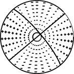
The mechanism correspond to the best fit is
|
|
Figure 1. Waveform inversion focal mechanism
|
The best fit as a function of depth is given in the following figure:
|
|
Figure 2. Depth sensitivity for waveform mechanism
|
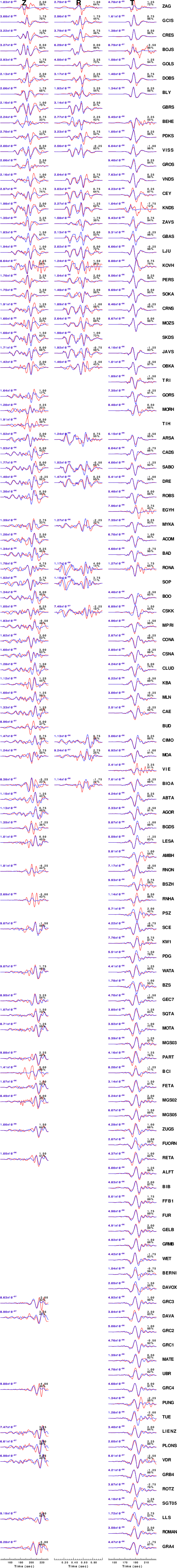
The comparison of the observed and predicted waveforms is given in the next figure. The red traces are the observed and the blue are the predicted.
Each observed-predicted component is plotted to the same scale and peak amplitudes are indicated by the numbers to the left of each trace. A pair of numbers is given in black at the right of each predicted traces. The upper number it the time shift required for maximum correlation between the observed and predicted traces. This time shift is required because the synthetics are not computed at exactly the same distance as the observed and because the velocity model used in the predictions may not be perfect.
A positive time shift indicates that the prediction is too fast and should be delayed to match the observed trace (shift to the right in this figure). A negative value indicates that the prediction is too slow. The lower number gives the percentage of variance reduction to characterize the individual goodness of fit (100% indicates a perfect fit).
The bandpass filter used in the processing and for the display was
cut o DIST/3.3 -40 o DIST/3.3 +50
rtr
taper w 0.1
hp c 0.03 n 3
lp c 0.06 n 3
|
|
Figure 3. Waveform comparison for selected depth
|
|
|
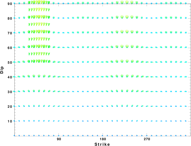
Focal mechanism sensitivity at the preferred depth. The red color indicates a very good fit to thewavefroms.
Each solution is plotted as a vector at a given value of strike and dip with the angle of the vector representing the rake angle, measured, with respect to the upward vertical (N) in the figure.
|
A check on the assumed source location is possible by looking at the time shifts between the observed and predicted traces. The time shifts for waveform matching arise for several reasons:
- The origin time and epicentral distance are incorrect
- The velocity model used for the inversion is incorrect
- The velocity model used to define the P-arrival time is not the
same as the velocity model used for the waveform inversion
(assuming that the initial trace alignment is based on the
P arrival time)
Assuming only a mislocation, the time shifts are fit to a functional form:
Time_shift = A + B cos Azimuth + C Sin Azimuth
The time shifts for this inversion lead to the next figure:
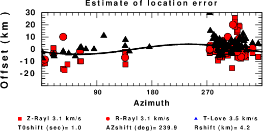
The derived shift in origin time and epicentral coordinates are given at the bottom of the figure.
Discussion
Acknowledgements
Thanks also to the many seismic network operators whose dedication make this effort possible: University of Nevada Reno, University of Alaska, University of Washington, Oregon State University, University of Utah, Montana Bureas of Mines, UC Berkely, Caltech, UC San Diego, Saint Louis University, University of Memphis, Lamont Doherty Earth Observatory, the Iris stations and the Transportable Array of EarthScope.
Velocity Model
The WUS.model used for the waveform synthetic seismograms and for the surface wave eigenfunctions and dispersion is as follows:
MODEL.01
Model after     8 iterations
ISOTROPIC
KGS
FLAT EARTH
1-D
CONSTANT VELOCITY
LINE08
LINE09
LINE10
LINE11
      H(KM)   VP(KM/S)   VS(KM/S) RHO(GM/CC)         QP         QS       ETAP       ETAS      FREFP      FREFS
     1.9000     3.4065     2.0089     2.2150  0.302E-02  0.679E-02   0.00       0.00       1.00       1.00
     6.1000     5.5445     3.2953     2.6089  0.349E-02  0.784E-02   0.00       0.00       1.00       1.00
    13.0000     6.2708     3.7396     2.7812  0.212E-02  0.476E-02   0.00       0.00       1.00       1.00
    19.0000     6.4075     3.7680     2.8223  0.111E-02  0.249E-02   0.00       0.00       1.00       1.00
     0.0000     7.9000     4.6200     3.2760  0.164E-10  0.370E-10   0.00       0.00       1.00       1.00
Quality Control
Here we tabulate the reasons for not using certain digital data sets
The following stations did not have a valid response files:
Last Changed Wed Jan 6 15:29:24 CST 2021