Location
Location ANSS
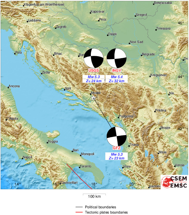
2019/11/26 09:19:26 43.20 17.96 10 5.4 Bosnia-Herzegovina
Focal Mechanism
 USGS/SLU Moment Tensor Solution
 ENS  2019/11/26 09:19:26:0  43.20   17.96  10.0 5.4 Bosnia-Herzegovina

 Stations used:
   AC.KBN HL.RDO HT.KAVA HT.KNT HT.OUR HT.SOH HT.SRS HT.THE
   HU.BEHE HU.KOVH HU.MORH HU.TIH IV.PTCC MN.BZS MN.PDG MN.TRI
   OX.ACOM OX.BAD OX.DRE OX.SABO SJ.BBLS SJ.FRGS

 Filtering commands used:
   cut o DIST/3.3 -30 o DIST/3.3 +70
   rtr
   taper w 0.1
   hp c 0.02 n 3
   lp c 0.10 n 3

 Best Fitting Double Couple
  Mo = 7.41e+23 dyne-cm
  Mw = 5.18
  Z  = 21 km
  Plane   Strike  Dip  Rake
   NP1      157    66   141
   NP2      265    55    30
  Principal Axes:
   Axis    Value   Plunge  Azimuth
    T   7.41e+23     44     117
    N   0.00e+00     45     310
    P  -7.41e+23      7     213

 Moment Tensor: (dyne-cm)
    Component   Value
       Mxx    -4.37e+23
       Mxy    -4.88e+23
       Mxz    -9.42e+22
       Myy     8.87e+22
       Myz     3.78e+23
       Mzz     3.48e+23


                     --------------
                 ##--------------------
              #####-----------------------
             ######------------------------
           ########--------------------------
          #########---------------------------
         ##########-----#############----------
        ##########--######################------
        ######------##########################--
       ####---------############################-
       ##------------############################
       #--------------###########################
       ----------------##############   #########
        ---------------############## T ########
        ----------------#############   ########
         ----------------######################
          -----------------###################
           -----------------#################
             --   ------------#############
              - P -------------###########
                  ----------------#####
                     --------------


 Global CMT Convention Moment Tensor:
      R          T          P
  3.48e+23  -9.42e+22  -3.78e+23
 -9.42e+22  -4.37e+23   4.88e+23
 -3.78e+23   4.88e+23   8.87e+22


Details of the solution is found at

http://www.eas.slu.edu/eqc/eqc_mt/MECH.NA/20191126091926/index.html
|
Preferred Solution
The preferred solution from an analysis of the surface-wave spectral amplitude radiation pattern, waveform inversion and first motion observations is
      STK = 265
      DIP = 55
     RAKE = 30
       MW = 5.18
       HS = 21.0
The NDK file is 20191126091926.ndk
The waveform inversion is preferred.
Moment Tensor Comparison
The following compares this source inversion to others
| SLU |
EMSC |
 USGS/SLU Moment Tensor Solution
 ENS  2019/11/26 09:19:26:0  43.20   17.96  10.0 5.4 Bosnia-Herzegovina

 Stations used:
   AC.KBN HL.RDO HT.KAVA HT.KNT HT.OUR HT.SOH HT.SRS HT.THE
   HU.BEHE HU.KOVH HU.MORH HU.TIH IV.PTCC MN.BZS MN.PDG MN.TRI
   OX.ACOM OX.BAD OX.DRE OX.SABO SJ.BBLS SJ.FRGS

 Filtering commands used:
   cut o DIST/3.3 -30 o DIST/3.3 +70
   rtr
   taper w 0.1
   hp c 0.02 n 3
   lp c 0.10 n 3

 Best Fitting Double Couple
  Mo = 7.41e+23 dyne-cm
  Mw = 5.18
  Z  = 21 km
  Plane   Strike  Dip  Rake
   NP1      157    66   141
   NP2      265    55    30
  Principal Axes:
   Axis    Value   Plunge  Azimuth
    T   7.41e+23     44     117
    N   0.00e+00     45     310
    P  -7.41e+23      7     213

 Moment Tensor: (dyne-cm)
    Component   Value
       Mxx    -4.37e+23
       Mxy    -4.88e+23
       Mxz    -9.42e+22
       Myy     8.87e+22
       Myz     3.78e+23
       Mzz     3.48e+23


                     --------------
                 ##--------------------
              #####-----------------------
             ######------------------------
           ########--------------------------
          #########---------------------------
         ##########-----#############----------
        ##########--######################------
        ######------##########################--
       ####---------############################-
       ##------------############################
       #--------------###########################
       ----------------##############   #########
        ---------------############## T ########
        ----------------#############   ########
         ----------------######################
          -----------------###################
           -----------------#################
             --   ------------#############
              - P -------------###########
                  ----------------#####
                     --------------


 Global CMT Convention Moment Tensor:
      R          T          P
  3.48e+23  -9.42e+22  -3.78e+23
 -9.42e+22  -4.37e+23   4.88e+23
 -3.78e+23   4.88e+23   8.87e+22


Details of the solution is found at

http://www.eas.slu.edu/eqc/eqc_mt/MECH.NA/20191126091926/index.html
|
Summary at EMSC-CSEM
|
Magnitudes
mLg Magnitude
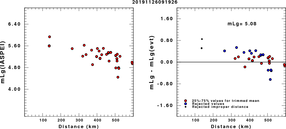
(a) mLg computed using the IASPEI formula; (b) mLg residuals ; the values used for the trimmed mean are indicated.
ML Magnitude
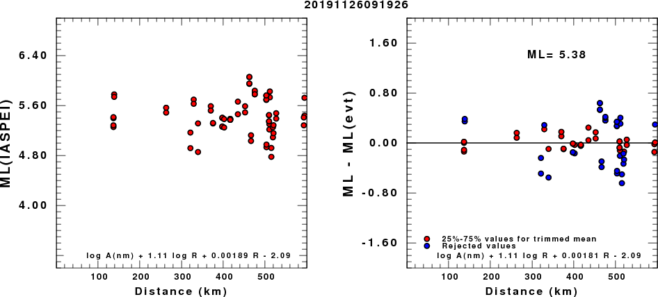
(a) ML computed using the IASPEI formula for Horizontal components; (b) ML residuals computed using a modified IASPEI formula that accounts for path specific attenuation; the values used for the trimmed mean are indicated. The ML relation used for each figure is given at the bottom of each plot.
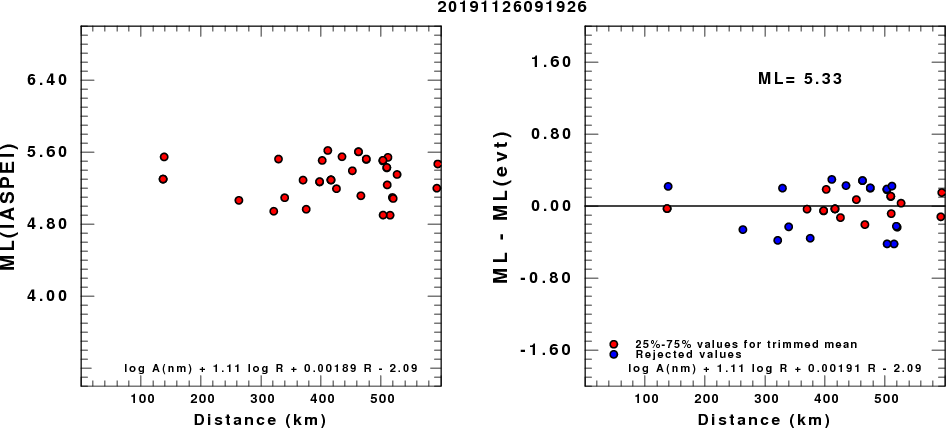
(a) ML computed using the IASPEI formula for Vertical components (research); (b) ML residuals computed using a modified IASPEI formula that accounts for path specific attenuation; the values used for the trimmed mean are indicated. The ML relation used for each figure is given at the bottom of each plot.
Waveform Inversion
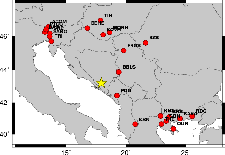
The focal mechanism was determined using broadband seismic waveforms. The location of the event and the
and stations used for the waveform inversion are shown in the next figure.
|
|
Location of broadband stations used for waveform inversion
|
The program wvfgrd96 was used with good traces observed at short distance to determine the focal mechanism, depth and seismic moment. This technique requires a high quality signal and well determined velocity model for the Green functions. To the extent that these are the quality data, this type of mechanism should be preferred over the radiation pattern technique which requires the separate step of defining the pressure and tension quadrants and the correct strike.
The observed and predicted traces are filtered using the following gsac commands:
cut o DIST/3.3 -30 o DIST/3.3 +70
rtr
taper w 0.1
hp c 0.02 n 3
lp c 0.10 n 3
The results of this grid search from 0.5 to 19 km depth are as follow:
           DEPTH  STK   DIP  RAKE   MW    FIT
WVFGRD96    1.0   160    60   -35   4.64 0.2515
WVFGRD96    2.0   125    45   -85   4.84 0.3497
WVFGRD96    3.0   335    50   -45   4.87 0.3651
WVFGRD96    4.0   355    80     0   4.86 0.3635
WVFGRD96    5.0   355    80     0   4.88 0.3492
WVFGRD96    6.0   165    90    35   4.85 0.3549
WVFGRD96    7.0   165    90    35   4.88 0.3826
WVFGRD96    8.0   345    90   -40   4.94 0.4074
WVFGRD96    9.0   345    90   -35   4.97 0.4304
WVFGRD96   10.0   345    90   -35   4.99 0.4496
WVFGRD96   11.0   345    90   -35   5.01 0.4655
WVFGRD96   12.0   345    90   -35   5.03 0.4774
WVFGRD96   13.0   340    80   -40   5.04 0.4854
WVFGRD96   14.0   340    80   -35   5.07 0.4902
WVFGRD96   15.0   340    80   -35   5.08 0.4907
WVFGRD96   16.0   260    55    20   5.09 0.5023
WVFGRD96   17.0   265    55    30   5.11 0.5129
WVFGRD96   18.0   265    55    30   5.13 0.5216
WVFGRD96   19.0   265    55    30   5.15 0.5282
WVFGRD96   20.0   265    55    30   5.16 0.5312
WVFGRD96   21.0   265    55    30   5.18 0.5333
WVFGRD96   22.0   265    55    30   5.19 0.5320
WVFGRD96   23.0   265    55    30   5.20 0.5266
WVFGRD96   24.0   265    55    30   5.21 0.5205
WVFGRD96   25.0   265    55    30   5.21 0.5105
WVFGRD96   26.0   265    60    30   5.22 0.5017
WVFGRD96   27.0   265    60    30   5.23 0.4900
WVFGRD96   28.0   265    60    30   5.24 0.4784
WVFGRD96   29.0    70    40    20   5.23 0.4662
The best solution is
WVFGRD96 21.0 265 55 30 5.18 0.5333
The mechanism correspond to the best fit is
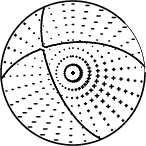
|
|
Figure 1. Waveform inversion focal mechanism
|
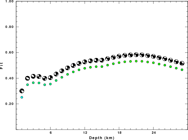
The best fit as a function of depth is given in the following figure:
|
|
Figure 2. Depth sensitivity for waveform mechanism
|
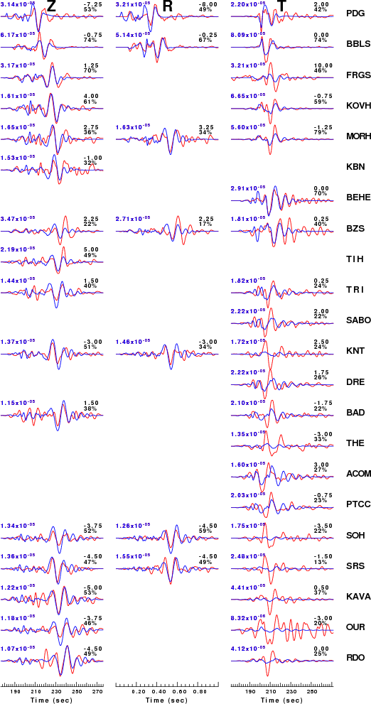
The comparison of the observed and predicted waveforms is given in the next figure. The red traces are the observed and the blue are the predicted.
Each observed-predicted component is plotted to the same scale and peak amplitudes are indicated by the numbers to the left of each trace. A pair of numbers is given in black at the right of each predicted traces. The upper number it the time shift required for maximum correlation between the observed and predicted traces. This time shift is required because the synthetics are not computed at exactly the same distance as the observed and because the velocity model used in the predictions may not be perfect.
A positive time shift indicates that the prediction is too fast and should be delayed to match the observed trace (shift to the right in this figure). A negative value indicates that the prediction is too slow. The lower number gives the percentage of variance reduction to characterize the individual goodness of fit (100% indicates a perfect fit).
The bandpass filter used in the processing and for the display was
cut o DIST/3.3 -30 o DIST/3.3 +70
rtr
taper w 0.1
hp c 0.02 n 3
lp c 0.10 n 3
|
|
Figure 3. Waveform comparison for selected depth
|
|
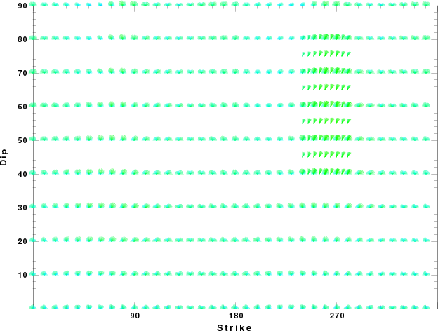
|
Focal mechanism sensitivity at the preferred depth. The red color indicates a very good fit to thewavefroms.
Each solution is plotted as a vector at a given value of strike and dip with the angle of the vector representing the rake angle, measured, with respect to the upward vertical (N) in the figure.
|
A check on the assumed source location is possible by looking at the time shifts between the observed and predicted traces. The time shifts for waveform matching arise for several reasons:
- The origin time and epicentral distance are incorrect
- The velocity model used for the inversion is incorrect
- The velocity model used to define the P-arrival time is not the
same as the velocity model used for the waveform inversion
(assuming that the initial trace alignment is based on the
P arrival time)
Assuming only a mislocation, the time shifts are fit to a functional form:
Time_shift = A + B cos Azimuth + C Sin Azimuth
The time shifts for this inversion lead to the next figure:
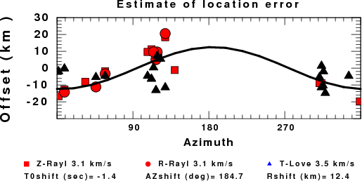
The derived shift in origin time and epicentral coordinates are given at the bottom of the figure.
Discussion
Acknowledgements
Thanks also to the many seismic network operators whose dedication make this effort possible: University of Nevada Reno, University of Alaska, University of Washington, Oregon State University, University of Utah, Montana Bureas of Mines, UC Berkely, Caltech, UC San Diego, Saint Louis University, University of Memphis, Lamont Doherty Earth Observatory, the Iris stations and the Transportable Array of EarthScope.
Velocity Model
The WUS used for the waveform synthetic seismograms and for the surface wave eigenfunctions and dispersion is as follows:
MODEL.01
Model after     8 iterations
ISOTROPIC
KGS
FLAT EARTH
1-D
CONSTANT VELOCITY
LINE08
LINE09
LINE10
LINE11
      H(KM)   VP(KM/S)   VS(KM/S) RHO(GM/CC)         QP         QS       ETAP       ETAS      FREFP      FREFS
     1.9000     3.4065     2.0089     2.2150  0.302E-02  0.679E-02   0.00       0.00       1.00       1.00
     6.1000     5.5445     3.2953     2.6089  0.349E-02  0.784E-02   0.00       0.00       1.00       1.00
    13.0000     6.2708     3.7396     2.7812  0.212E-02  0.476E-02   0.00       0.00       1.00       1.00
    19.0000     6.4075     3.7680     2.8223  0.111E-02  0.249E-02   0.00       0.00       1.00       1.00
     0.0000     7.9000     4.6200     3.2760  0.164E-10  0.370E-10   0.00       0.00       1.00       1.00
Quality Control
Here we tabulate the reasons for not using certain digital data sets
The following stations did not have a valid response files:
Last Changed Tue Nov 26 08:44:37 CST 2019