Location

Location ANSS

Focal Mechanism

USGS/SLU Moment Tensor Solution ENS 2019/11/26 02:54:11:0 41.45 19.44 10.0 6.4 Albania Stations used: AC.KBN BS.ELND BS.LOZB BS.PLVB BS.RAZG CL.PSAM CL.TRIZ HA.ATAL HA.AXAR HA.LOUT HA.MAGU HA.MAKR HA.STFN HL.ATH HL.DION HL.EVR HL.KZN HL.LIA HL.LKR HL.NEO HL.PENT HL.PRK HL.PTL HL.RDO HL.SKY HL.SMTH HL.VLY HP.AMPL HP.GUR HP.PRMD HT.HORT HT.IGT HT.KAVA HT.KNT HT.LIT HT.NEST HT.OUR HT.SIGR HT.SOH HT.SRS HT.THE HT.TYRN HU.BEHE HU.BUD HU.KOVH HU.MORH KO.ERIK KO.GADA KO.LAP MN.BZS MN.PDG MN.TRI RO.BAIL RO.BZS RO.COPA RO.DEV RO.DRGR RO.GZR RO.HERR RO.HUMR RO.LOT RO.MDVR RO.PUNG RO.SIRR RO.VLAD SJ.BBLS SJ.FRGS Filtering commands used: cut o DIST/3.3 -20 o DIST/3.3 +80 rtr taper w 0.1 hp c 0.02 n 3 lp c 0.06 n 3 Best Fitting Double Couple Mo = 3.09e+25 dyne-cm Mw = 6.26 Z = 31 km Plane Strike Dip Rake NP1 136 77 98 NP2 285 15 60 Principal Axes: Axis Value Plunge Azimuth T 3.09e+25 57 56 N 0.00e+00 7 314 P -3.09e+25 32 220 Moment Tensor: (dyne-cm) Component Value Mxx -1.05e+25 Mxy -6.81e+24 Mxz 1.85e+25 Myy -2.90e+24 Myz 2.04e+25 Mzz 1.34e+25 -------------- ------########-------- ----###################----- #-#########################--- #---###########################--- #-----############################-- --------############################-- ----------############### ##########-- ------------############# T ###########- --------------############ ###########-- ----------------#########################- -----------------########################- -------------------######################- --------------------#################### ----------------------################## --------- -----------############### -------- P -------------############ ------- ----------------######## ---------------------------### ---------------------------- ---------------------- -------------- Global CMT Convention Moment Tensor: R T P 1.34e+25 1.85e+25 -2.04e+25 1.85e+25 -1.05e+25 6.81e+24 -2.04e+25 6.81e+24 -2.90e+24 Details of the solution is found at http://www.eas.slu.edu/eqc/eqc_mt/MECH.NA/20191126025411/index.html

Preferred Solution

      STK = 285
      DIP = 15
     RAKE = 60
       MW = 6.26
       HS = 31.0

The NDK file is 20191126025411.ndk The waveform inversion is preferred.

Moment Tensor Comparison

The following compares this source inversion to others

SLU	USGSW	EMSC
USGS/SLU Moment Tensor Solution ENS 2019/11/26 02:54:11:0 41.45 19.44 10.0 6.4 Albania Stations used: AC.KBN BS.ELND BS.LOZB BS.PLVB BS.RAZG CL.PSAM CL.TRIZ HA.ATAL HA.AXAR HA.LOUT HA.MAGU HA.MAKR HA.STFN HL.ATH HL.DION HL.EVR HL.KZN HL.LIA HL.LKR HL.NEO HL.PENT HL.PRK HL.PTL HL.RDO HL.SKY HL.SMTH HL.VLY HP.AMPL HP.GUR HP.PRMD HT.HORT HT.IGT HT.KAVA HT.KNT HT.LIT HT.NEST HT.OUR HT.SIGR HT.SOH HT.SRS HT.THE HT.TYRN HU.BEHE HU.BUD HU.KOVH HU.MORH KO.ERIK KO.GADA KO.LAP MN.BZS MN.PDG MN.TRI RO.BAIL RO.BZS RO.COPA RO.DEV RO.DRGR RO.GZR RO.HERR RO.HUMR RO.LOT RO.MDVR RO.PUNG RO.SIRR RO.VLAD SJ.BBLS SJ.FRGS Filtering commands used: cut o DIST/3.3 -20 o DIST/3.3 +80 rtr taper w 0.1 hp c 0.02 n 3 lp c 0.06 n 3 Best Fitting Double Couple Mo = 3.09e+25 dyne-cm Mw = 6.26 Z = 31 km Plane Strike Dip Rake NP1 136 77 98 NP2 285 15 60 Principal Axes: Axis Value Plunge Azimuth T 3.09e+25 57 56 N 0.00e+00 7 314 P -3.09e+25 32 220 Moment Tensor: (dyne-cm) Component Value Mxx -1.05e+25 Mxy -6.81e+24 Mxz 1.85e+25 Myy -2.90e+24 Myz 2.04e+25 Mzz 1.34e+25 -------------- ------########-------- ----###################----- #-#########################--- #---###########################--- #-----############################-- --------############################-- ----------############### ##########-- ------------############# T ###########- --------------############ ###########-- ----------------#########################- -----------------########################- -------------------######################- --------------------#################### ----------------------################## --------- -----------############### -------- P -------------############ ------- ----------------######## ---------------------------### ---------------------------- ---------------------- -------------- Global CMT Convention Moment Tensor: R T P 1.34e+25 1.85e+25 -2.04e+25 1.85e+25 -1.05e+25 6.81e+24 -2.04e+25 6.81e+24 -2.90e+24 Details of the solution is found at http://www.eas.slu.edu/eqc/eqc_mt/MECH.NA/20191126025411/index.html	W-phase Moment Tensor (Mww) Moment 4.561e+18 N-m Magnitude 6.37 Mww Depth 19.5 km Percent DC 78% Half Duration 3.89 s Catalog US Data Source US 2 Contributor US 2 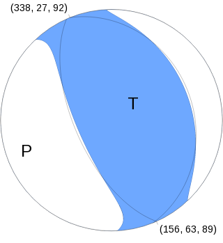Nodal Planes Plane Strike Dip Rake NP1 338Â 27Â 92Â NP2 156Â 63Â 89Â Principal Axes Axis Value Plunge Azimuth T 4.269e+18 N-m 72Â 64Â N 0.538e+18 N-m 1Â 156Â P -4.806e+18 N-m 18Â 247Â	EMSC-CSEM Solutions

Magnitudes

mLg Magnitude

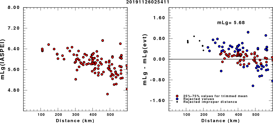
(a) mLg computed using the IASPEI formula; (b) mLg residuals ; the values used for the trimmed mean are indicated.

ML Magnitude

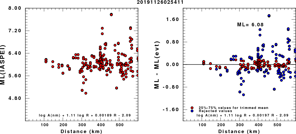
(a) ML computed using the IASPEI formula for Horizontal components; (b) ML residuals computed using a modified IASPEI formula that accounts for path specific attenuation; the values used for the trimmed mean are indicated. The ML relation used for each figure is given at the bottom of each plot.

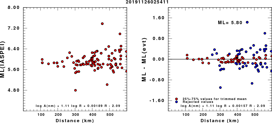
(a) ML computed using the IASPEI formula for Vertical components (research); (b) ML residuals computed using a modified IASPEI formula that accounts for path specific attenuation; the values used for the trimmed mean are indicated. The ML relation used for each figure is given at the bottom of each plot.

Waveform Inversion

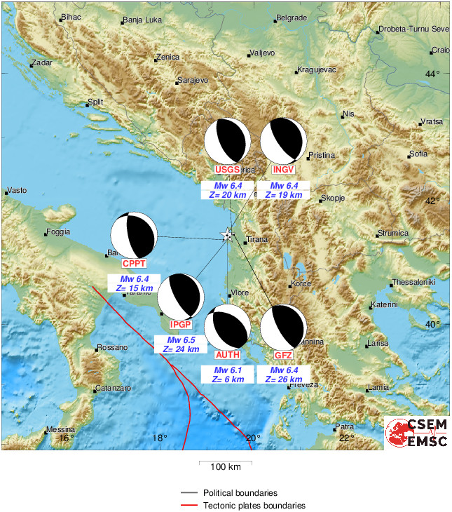
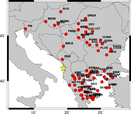
The focal mechanism was determined using broadband seismic waveforms. The location of the event and the and stations used for the waveform inversion are shown in the next figure.

Location of broadband stations used for waveform inversion

The program wvfgrd96 was used with good traces observed at short distance to determine the focal mechanism, depth and seismic moment. This technique requires a high quality signal and well determined velocity model for the Green functions. To the extent that these are the quality data, this type of mechanism should be preferred over the radiation pattern technique which requires the separate step of defining the pressure and tension quadrants and the correct strike.

The observed and predicted traces are filtered using the following gsac commands:

cut o DIST/3.3 -20 o DIST/3.3 +80
rtr
taper w 0.1
hp c 0.02 n 3 
lp c 0.06 n 3 

           DEPTH  STK   DIP  RAKE   MW    FIT
WVFGRD96    1.0   140    45   -90   5.81 0.2446
WVFGRD96    2.0   140    45   -90   5.90 0.3039
WVFGRD96    3.0   320    45   -90   5.93 0.2813
WVFGRD96    4.0    55    45    75   5.89 0.2477
WVFGRD96    5.0    35    50    50   5.87 0.2368
WVFGRD96    6.0   190    35    -5   5.88 0.2527
WVFGRD96    7.0   190    35    -5   5.89 0.2738
WVFGRD96    8.0   175    20   -40   6.01 0.2962
WVFGRD96    9.0   165    15   -60   6.05 0.3306
WVFGRD96   10.0   275    15    50   6.06 0.3640
WVFGRD96   11.0   275    15    50   6.08 0.3956
WVFGRD96   12.0   285    15    60   6.09 0.4237
WVFGRD96   13.0   275    15    50   6.10 0.4485
WVFGRD96   14.0   285    15    60   6.11 0.4719
WVFGRD96   15.0   285    15    60   6.12 0.4921
WVFGRD96   16.0   290    15    65   6.13 0.5102
WVFGRD96   17.0   290    15    65   6.14 0.5268
WVFGRD96   18.0   285    15    60   6.15 0.5417
WVFGRD96   19.0   285    15    60   6.16 0.5551
WVFGRD96   20.0   275    20    50   6.17 0.5672
WVFGRD96   21.0   285    15    60   6.19 0.5783
WVFGRD96   22.0   285    15    60   6.19 0.5880
WVFGRD96   23.0   285    15    60   6.20 0.5965
WVFGRD96   24.0   285    15    60   6.21 0.6039
WVFGRD96   25.0   285    15    60   6.22 0.6104
WVFGRD96   26.0   285    15    60   6.23 0.6160
WVFGRD96   27.0   285    15    60   6.24 0.6206
WVFGRD96   28.0   285    15    60   6.24 0.6241
WVFGRD96   29.0   285    15    60   6.25 0.6266
WVFGRD96   30.0   285    15    60   6.26 0.6280
WVFGRD96   31.0   285    15    60   6.26 0.6283
WVFGRD96   32.0   290    15    65   6.27 0.6276
WVFGRD96   33.0   290    15    65   6.28 0.6259
WVFGRD96   34.0   280    20    55   6.28 0.6233
WVFGRD96   35.0   285    20    60   6.29 0.6199
WVFGRD96   36.0   285    20    60   6.29 0.6156
WVFGRD96   37.0   285    20    60   6.29 0.6104
WVFGRD96   38.0   290    20    65   6.30 0.6046
WVFGRD96   39.0   295    20    70   6.30 0.5985

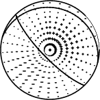
The best solution is

WVFGRD96   31.0   285    15    60   6.26 0.6283

The mechanism correspond to the best fit is

Figure 1. Waveform inversion focal mechanism

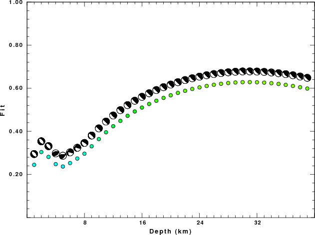
The best fit as a function of depth is given in the following figure:

Figure 2. Depth sensitivity for waveform mechanism

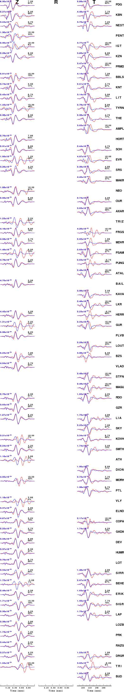
The comparison of the observed and predicted waveforms is given in the next figure. The red traces are the observed and the blue are the predicted. Each observed-predicted component is plotted to the same scale and peak amplitudes are indicated by the numbers to the left of each trace. A pair of numbers is given in black at the right of each predicted traces. The upper number it the time shift required for maximum correlation between the observed and predicted traces. This time shift is required because the synthetics are not computed at exactly the same distance as the observed and because the velocity model used in the predictions may not be perfect. A positive time shift indicates that the prediction is too fast and should be delayed to match the observed trace (shift to the right in this figure). A negative value indicates that the prediction is too slow. The lower number gives the percentage of variance reduction to characterize the individual goodness of fit (100% indicates a perfect fit).

The bandpass filter used in the processing and for the display was

cut o DIST/3.3 -20 o DIST/3.3 +80
rtr
taper w 0.1
hp c 0.02 n 3 
lp c 0.06 n 3 

Figure 3. Waveform comparison for selected depth

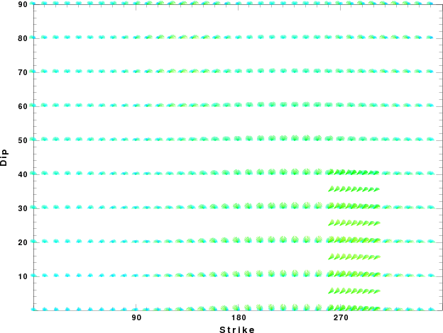
Focal mechanism sensitivity at the preferred depth. The red color indicates a very good fit to thewavefroms. Each solution is plotted as a vector at a given value of strike and dip with the angle of the vector representing the rake angle, measured, with respect to the upward vertical (N) in the figure.

A check on the assumed source location is possible by looking at the time shifts between the observed and predicted traces. The time shifts for waveform matching arise for several reasons:

• The origin time and epicentral distance are incorrect
• The velocity model used for the inversion is incorrect
• The velocity model used to define the P-arrival time is not the same as the velocity model used for the waveform inversion (assuming that the initial trace alignment is based on the P arrival time)

 Time_shift = A + B cos Azimuth + C Sin Azimuth

The time shifts for this inversion lead to the next figure:

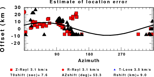
The derived shift in origin time and epicentral coordinates are given at the bottom of the figure.

Discussion

Acknowledgements

Thanks also to the many seismic network operators whose dedication make this effort possible: University of Nevada Reno, University of Alaska, University of Washington, Oregon State University, University of Utah, Montana Bureas of Mines, UC Berkely, Caltech, UC San Diego, Saint Louis University, University of Memphis, Lamont Doherty Earth Observatory, the Iris stations and the Transportable Array of EarthScope.

Velocity Model

The WUS used for the waveform synthetic seismograms and for the surface wave eigenfunctions and dispersion is as follows:

MODEL.01
Model after     8 iterations
ISOTROPIC
KGS
FLAT EARTH
1-D
CONSTANT VELOCITY
LINE08
LINE09
LINE10
LINE11
      H(KM)   VP(KM/S)   VS(KM/S) RHO(GM/CC)         QP         QS       ETAP       ETAS      FREFP      FREFS
     1.9000     3.4065     2.0089     2.2150  0.302E-02  0.679E-02   0.00       0.00       1.00       1.00    
     6.1000     5.5445     3.2953     2.6089  0.349E-02  0.784E-02   0.00       0.00       1.00       1.00    
    13.0000     6.2708     3.7396     2.7812  0.212E-02  0.476E-02   0.00       0.00       1.00       1.00    
    19.0000     6.4075     3.7680     2.8223  0.111E-02  0.249E-02   0.00       0.00       1.00       1.00    
     0.0000     7.9000     4.6200     3.2760  0.164E-10  0.370E-10   0.00       0.00       1.00       1.00    

Quality Control

Here we tabulate the reasons for not using certain digital data sets

The following stations did not have a valid response files: