Location
Location ANSS
2019/11/11 10:52:45 44.54 4.63 10.0 4.9 France
Focal Mechanism
 USGS/SLU Moment Tensor Solution
 ENS  2019/11/11 10:52:45:0  44.54    4.63  10.0 4.9 France

 Stations used:
   FR.ARBF FR.ARTF FR.ATE FR.BSTF FR.CALF FR.CARF FR.CFF
   FR.CHMF FR.EILF FR.ESCA FR.FILF FR.FNEB FR.HOHE FR.ILLF
   FR.ISO FR.LABF FR.LRVF FR.MLS FR.MLYF FR.MONQ FR.PAND
   FR.PYLO FR.RUSF FR.SALF FR.SAOF FR.SPIF FR.TURF FR.URDF
   FR.VIEF FR.WLS FR.ZELS GE.STU GE.WLF GU.BHB GU.ENR GU.GBOS
   GU.GORR GU.PCP GU.POPM GU.PZZ GU.RORO GU.RRL GU.RSP GU.SATI
   GU.STV IV.BDI IV.IMI IV.MONC IV.MSSA IV.PLMA IV.QLNO MN.BNI
   MN.TUE MN.VLC RD.LOR RD.MTLF RD.ORIF

 Filtering commands used:
   cut o DIST/3.3 -30 o DIST/3.3 +60
   rtr
   taper w 0.1
   hp c 0.02 n 3
   lp c 0.06 n 3

 Best Fitting Double Couple
  Mo = 2.37e+23 dyne-cm
  Mw = 4.85
  Z  = 22 km
  Plane   Strike  Dip  Rake
   NP1       65    59   106
   NP2      215    35    65
  Principal Axes:
   Axis    Value   Plunge  Azimuth
    T   2.37e+23     71      13
    N   0.00e+00     14     236
    P  -2.37e+23     12     143

 Moment Tensor: (dyne-cm)
    Component   Value
       Mxx    -1.20e+23
       Mxy     1.15e+23
       Mxz     1.09e+23
       Myy    -8.15e+22
       Myz    -1.31e+22
       Mzz     2.02e+23


                     --------------
                 ----------------####--
              ------------################
             ----------####################
           ----------########################
          ---------###########################
         --------##############################
        --------############   ###############--
        -------############# T ##############---
       -------##############   #############-----
       -------############################-------
       ------############################--------
       ------#########################-----------
        -----#######################------------
        -----####################---------------
         ----################------------------
          ############------------------------
           ###------------------------   ----
             #------------------------ P --
              #-----------------------   -
                 ----------------------
                     --------------


 Global CMT Convention Moment Tensor:
      R          T          P
  2.02e+23   1.09e+23   1.31e+22
  1.09e+23  -1.20e+23  -1.15e+23
  1.31e+22  -1.15e+23  -8.15e+22


Details of the solution is found at

http://www.eas.slu.edu/eqc/eqc_mt/MECH.NA/20191111105245/index.html
|
Preferred Solution
The preferred solution from an analysis of the surface-wave spectral amplitude radiation pattern, waveform inversion and first motion observations is
      STK = 215
      DIP = 35
     RAKE = 65
       MW = 4.85
       HS = 22.0
The NDK file is 20191111105245.ndk
Depth control was not good originally. However the moment tensor solution agrees with first motions. The depth for the RMT depends on the velocity model. This was not easy.
Moment Tensor Comparison
The following compares this source inversion to others
| SLU |
SLUFM |
GFZ |
OCA |
 USGS/SLU Moment Tensor Solution
 ENS  2019/11/11 10:52:45:0  44.54    4.63  10.0 4.9 France

 Stations used:
   FR.ARBF FR.ARTF FR.ATE FR.BSTF FR.CALF FR.CARF FR.CFF
   FR.CHMF FR.EILF FR.ESCA FR.FILF FR.FNEB FR.HOHE FR.ILLF
   FR.ISO FR.LABF FR.LRVF FR.MLS FR.MLYF FR.MONQ FR.PAND
   FR.PYLO FR.RUSF FR.SALF FR.SAOF FR.SPIF FR.TURF FR.URDF
   FR.VIEF FR.WLS FR.ZELS GE.STU GE.WLF GU.BHB GU.ENR GU.GBOS
   GU.GORR GU.PCP GU.POPM GU.PZZ GU.RORO GU.RRL GU.RSP GU.SATI
   GU.STV IV.BDI IV.IMI IV.MONC IV.MSSA IV.PLMA IV.QLNO MN.BNI
   MN.TUE MN.VLC RD.LOR RD.MTLF RD.ORIF

 Filtering commands used:
   cut o DIST/3.3 -30 o DIST/3.3 +60
   rtr
   taper w 0.1
   hp c 0.02 n 3
   lp c 0.06 n 3

 Best Fitting Double Couple
  Mo = 2.37e+23 dyne-cm
  Mw = 4.85
  Z  = 22 km
  Plane   Strike  Dip  Rake
   NP1       65    59   106
   NP2      215    35    65
  Principal Axes:
   Axis    Value   Plunge  Azimuth
    T   2.37e+23     71      13
    N   0.00e+00     14     236
    P  -2.37e+23     12     143

 Moment Tensor: (dyne-cm)
    Component   Value
       Mxx    -1.20e+23
       Mxy     1.15e+23
       Mxz     1.09e+23
       Myy    -8.15e+22
       Myz    -1.31e+22
       Mzz     2.02e+23


                     --------------
                 ----------------####--
              ------------################
             ----------####################
           ----------########################
          ---------###########################
         --------##############################
        --------############   ###############--
        -------############# T ##############---
       -------##############   #############-----
       -------############################-------
       ------############################--------
       ------#########################-----------
        -----#######################------------
        -----####################---------------
         ----################------------------
          ############------------------------
           ###------------------------   ----
             #------------------------ P --
              #-----------------------   -
                 ----------------------
                     --------------


 Global CMT Convention Moment Tensor:
      R          T          P
  2.02e+23   1.09e+23   1.31e+22
  1.09e+23  -1.20e+23  -1.15e+23
  1.31e+22  -1.15e+23  -8.15e+22


Details of the solution is found at

http://www.eas.slu.edu/eqc/eqc_mt/MECH.NA/20191111105245/index.html
|
First motions and takeoff angles from an elocate run.
|
GFZ Event gfz2019wcnm
19/11/11 10:52:45.50
France
Epicenter: 44.59 4.65
MW 4.9

GFZ MOMENT TENSOR SOLUTION
Depth  13         No. of sta: 20
Moment Tensor;   Scale 10**16 Nm
  Mrr= 2.67       Mtt=-0.94
  Mpp=-1.73       Mrt=-0.05
  Mrp= 0.43       Mtp=-0.87
Principal axes:
  T  Val=  2.72  Plg=84  Azm=249
  N       -0.40       5       32
  P       -2.32       4      122

Best Double Couple:Mo=2.5*10**16
 NP1:Strike=218 Dip=41 Slip=  98
 NP2:        27     49        83

           -----------
        ----------------#
     -------------#######---
    -----------##########----
  ----------##############-----
  --------################-----
 --------#################------
--------##################-------
-------#######   ########--------
------######## T ########--------
------########   #######---------
-----###################---------
 ----##################---------
  ---################----------
  ---###############-----------
    --############-----------
     -#########-------------
        ####-------------
           -----------


Analysis performed by J. Saul
Last updated 2019-11-11 11:03:38 UTC
|
 Click here for OCA solution
http://sismoazur.oca.eu/resource/file?name=mwfm/result_complete.jpg&eventid=EMSC20191111105245
|
Magnitudes
mLg Magnitude
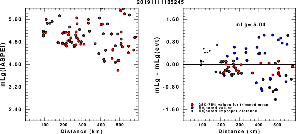
(a) mLg computed using the IASPEI formula; (b) mLg residuals ; the values used for the trimmed mean are indicated.
ML Magnitude
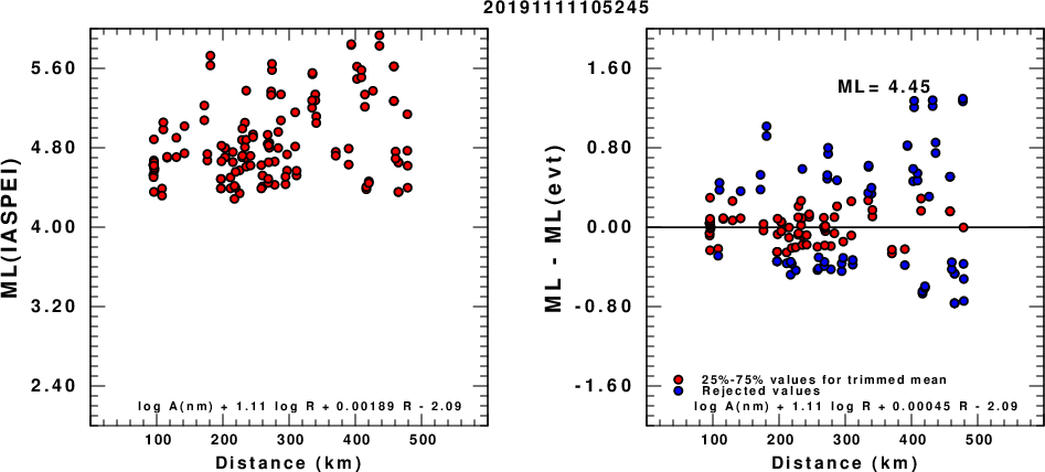
(a) ML computed using the IASPEI formula for Horizontal components; (b) ML residuals computed using a modified IASPEI formula that accounts for path specific attenuation; the values used for the trimmed mean are indicated. The ML relation used for each figure is given at the bottom of each plot.
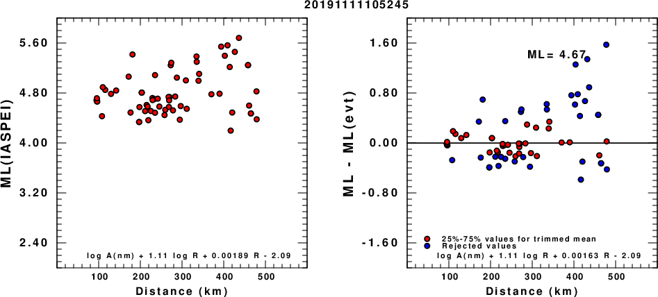
(a) ML computed using the IASPEI formula for Vertical components (research); (b) ML residuals computed using a modified IASPEI formula that accounts for path specific attenuation; the values used for the trimmed mean are indicated. The ML relation used for each figure is given at the bottom of each plot.
Context
The next figure presents the focal mechanism for this earthquake (red) in the context of other events (blue) in the SLU Moment Tensor Catalog which are within ± 0.5 degrees of the new event. This comparison is shown in the left panel of the figure. The right panel shows the inferred direction of maximum compressive stress and the type of faulting (green is strike-slip, red is normal, blue is thrust; oblique is shown by a combination of colors).
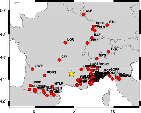
Waveform Inversion
The focal mechanism was determined using broadband seismic waveforms. The location of the event and the
and stations used for the waveform inversion are shown in the next figure.
|
|
Location of broadband stations used for waveform inversion
|
The program wvfgrd96 was used with good traces observed at short distance to determine the focal mechanism, depth and seismic moment. This technique requires a high quality signal and well determined velocity model for the Green functions. To the extent that these are the quality data, this type of mechanism should be preferred over the radiation pattern technique which requires the separate step of defining the pressure and tension quadrants and the correct strike.
The observed and predicted traces are filtered using the following gsac commands:
cut o DIST/3.3 -30 o DIST/3.3 +60
rtr
taper w 0.1
hp c 0.02 n 3
lp c 0.06 n 3
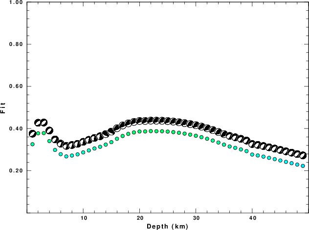
The results of this grid search from 0.5 to 19 km depth are as follow:
           DEPTH  STK   DIP  RAKE   MW    FIT
WVFGRD96    1.0   235    45   -80   4.54 0.3256
WVFGRD96    2.0    45    40   -95   4.63 0.3774
WVFGRD96    3.0    45    45   -95   4.69 0.3784
WVFGRD96    4.0   230    40   -80   4.72 0.3406
WVFGRD96    5.0   250    40   -55   4.70 0.2985
WVFGRD96    6.0   260    40   -35   4.67 0.2785
WVFGRD96    7.0   265    45   -25   4.66 0.2679
WVFGRD96    8.0   265    35   -25   4.71 0.2721
WVFGRD96    9.0   270    30   -15   4.70 0.2776
WVFGRD96   10.0   275    30   -10   4.70 0.2870
WVFGRD96   11.0   275    30   -10   4.71 0.2964
WVFGRD96   12.0   280    35     0   4.72 0.3055
WVFGRD96   13.0   280    35     0   4.72 0.3135
WVFGRD96   14.0   115    60    70   4.83 0.3238
WVFGRD96   15.0   115    60    70   4.83 0.3355
WVFGRD96   16.0   215    35    65   4.81 0.3515
WVFGRD96   17.0   215    35    65   4.82 0.3647
WVFGRD96   18.0   210    35    60   4.82 0.3746
WVFGRD96   19.0   210    35    60   4.83 0.3815
WVFGRD96   20.0   210    35    60   4.84 0.3860
WVFGRD96   21.0   215    35    65   4.85 0.3862
WVFGRD96   22.0   215    35    65   4.85 0.3877
WVFGRD96   23.0   210    35    60   4.86 0.3874
WVFGRD96   24.0   210    40    60   4.86 0.3871
WVFGRD96   25.0   210    40    60   4.86 0.3856
WVFGRD96   26.0   215    40    65   4.87 0.3831
WVFGRD96   27.0   215    40    65   4.87 0.3800
WVFGRD96   28.0   215    40    65   4.87 0.3759
WVFGRD96   29.0   210    45    60   4.88 0.3712
WVFGRD96   30.0   210    45    60   4.88 0.3658
WVFGRD96   31.0   215    45    65   4.88 0.3592
WVFGRD96   32.0   215    45    65   4.89 0.3516
WVFGRD96   33.0   215    45    65   4.89 0.3430
WVFGRD96   34.0   215    50    70   4.89 0.3338
WVFGRD96   35.0   215    50    70   4.89 0.3237
WVFGRD96   36.0   260    40   -40   4.91 0.3150
WVFGRD96   37.0   260    40   -40   4.92 0.3085
WVFGRD96   38.0   260    40   -45   4.92 0.3011
WVFGRD96   39.0   255    40   -50   4.93 0.2930
WVFGRD96   40.0   260    35   -40   5.03 0.2767
WVFGRD96   41.0   255    35   -45   5.04 0.2724
WVFGRD96   42.0   255    35   -45   5.04 0.2670
WVFGRD96   43.0   250    35   -55   5.05 0.2611
WVFGRD96   44.0   250    35   -55   5.05 0.2551
WVFGRD96   45.0   250    35   -55   5.06 0.2485
WVFGRD96   46.0   250    40   -55   5.06 0.2420
WVFGRD96   47.0   250    40   -55   5.07 0.2357
WVFGRD96   48.0   245    40   -65   5.07 0.2291
WVFGRD96   49.0   245    40   -65   5.07 0.2229
The best solution is
WVFGRD96 22.0 215 35 65 4.85 0.3877
The mechanism correspond to the best fit is
|
|
Figure 1. Waveform inversion focal mechanism
|
The best fit as a function of depth is given in the following figure:
|
|
Figure 2. Depth sensitivity for waveform mechanism
|
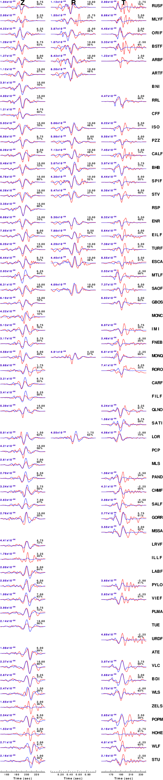
The comparison of the observed and predicted waveforms is given in the next figure. The red traces are the observed and the blue are the predicted.
Each observed-predicted component is plotted to the same scale and peak amplitudes are indicated by the numbers to the left of each trace. A pair of numbers is given in black at the right of each predicted traces. The upper number it the time shift required for maximum correlation between the observed and predicted traces. This time shift is required because the synthetics are not computed at exactly the same distance as the observed and because the velocity model used in the predictions may not be perfect.
A positive time shift indicates that the prediction is too fast and should be delayed to match the observed trace (shift to the right in this figure). A negative value indicates that the prediction is too slow. The lower number gives the percentage of variance reduction to characterize the individual goodness of fit (100% indicates a perfect fit).
The bandpass filter used in the processing and for the display was
cut o DIST/3.3 -30 o DIST/3.3 +60
rtr
taper w 0.1
hp c 0.02 n 3
lp c 0.06 n 3
|
|
Figure 3. Waveform comparison for selected depth
|
|
|
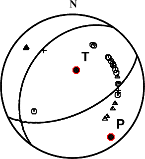
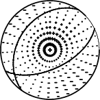
Focal mechanism sensitivity at the preferred depth. The red color indicates a very good fit to thewavefroms.
Each solution is plotted as a vector at a given value of strike and dip with the angle of the vector representing the rake angle, measured, with respect to the upward vertical (N) in the figure.
|
A check on the assumed source location is possible by looking at the time shifts between the observed and predicted traces. The time shifts for waveform matching arise for several reasons:
- The origin time and epicentral distance are incorrect
- The velocity model used for the inversion is incorrect
- The velocity model used to define the P-arrival time is not the
same as the velocity model used for the waveform inversion
(assuming that the initial trace alignment is based on the
P arrival time)
Assuming only a mislocation, the time shifts are fit to a functional form:
Time_shift = A + B cos Azimuth + C Sin Azimuth
The time shifts for this inversion lead to the next figure:
The derived shift in origin time and epicentral coordinates are given at the bottom of the figure.
Discussion
Acknowledgements
Thanks also to the many seismic network operators whose dedication make this effort possible: University of Nevada Reno, University of Alaska, University of Washington, Oregon State University, University of Utah, Montana Bureas of Mines, UC Berkely, Caltech, UC San Diego, Saint Louis University, University of Memphis, Lamont Doherty Earth Observatory, the Iris stations and the Transportable Array of EarthScope.
Velocity Model
The WUS.model used for the waveform synthetic seismograms and for the surface wave eigenfunctions and dispersion is as follows:
MODEL.01
Model after     8 iterations
ISOTROPIC
KGS
FLAT EARTH
1-D
CONSTANT VELOCITY
LINE08
LINE09
LINE10
LINE11
      H(KM)   VP(KM/S)   VS(KM/S) RHO(GM/CC)         QP         QS       ETAP       ETAS      FREFP      FREFS
     1.9000     3.4065     2.0089     2.2150  0.302E-02  0.679E-02   0.00       0.00       1.00       1.00
     6.1000     5.5445     3.2953     2.6089  0.349E-02  0.784E-02   0.00       0.00       1.00       1.00
    13.0000     6.2708     3.7396     2.7812  0.212E-02  0.476E-02   0.00       0.00       1.00       1.00
    19.0000     6.4075     3.7680     2.8223  0.111E-02  0.249E-02   0.00       0.00       1.00       1.00
     0.0000     7.9000     4.6200     3.2760  0.164E-10  0.370E-10   0.00       0.00       1.00       1.00
Quality Control
Here we tabulate the reasons for not using certain digital data sets
The following stations did not have a valid response files:
Last Changed Tue Nov 12 08:34:30 CST 2019