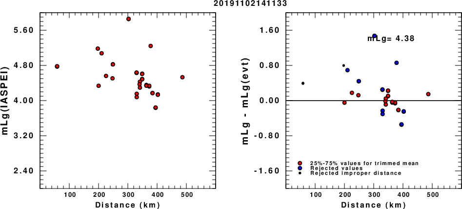
(a) mLg computed using the IASPEI formula; (b) mLg residuals ; the values used for the trimmed mean are indicated.
 USGS/SLU Moment Tensor Solution
 ENS  2019/11/02 14:11:33:5  44.32   17.61  10.0 4.7 Bosnia-Herzegovina

 Stations used:
   AC.KBN CR.ZAG HU.BEHE HU.KOVH HU.MORH MN.BLY MN.PDG MN.TRI
   OE.MYKA OE.OBKA OE.SOKA OX.DRE OX.PRED OX.SABO RO.BZS
   RO.MDVR RO.SIRR SJ.FRGS

 Filtering commands used:
   cut o DIST/3.3 -30 o DIST/3.3 +70
   rtr
   taper w 0.1
   hp c 0.02 n 3
   lp c 0.06 n 3

 Best Fitting Double Couple
  Mo = 1.86e+23 dyne-cm
  Mw = 4.78
  Z  = 18 km
  Plane   Strike  Dip  Rake
   NP1      235    65   -30
   NP2      339    63   -152
  Principal Axes:
   Axis    Value   Plunge  Azimuth
    T   1.86e+23      1     287
    N   0.00e+00     52      19
    P  -1.86e+23     38     196

 Moment Tensor: (dyne-cm)
    Component   Value
       Mxx    -8.95e+22
       Mxy    -8.35e+22
       Mxz     8.81e+22
       Myy     1.61e+23
       Myz     2.15e+22
       Mzz    -7.13e+22


                     --------------
                 #######---------------
              ############----------------
             ###############---------------
           ##################-------------##-
          ####################----############
          ###################---###############
        T ################-------###############
          ##############---------###############
       ##############-------------###############
       ############----------------##############
       ##########-------------------#############
       #########--------------------#############
        ######----------------------############
        #####------------------------###########
         ###-------------------------##########
          #------------   -----------#########
           ------------ P -----------########
             ----------   -----------######
              -----------------------#####
                 -------------------###
                     --------------


 Global CMT Convention Moment Tensor:
      R          T          P
 -7.13e+22   8.81e+22  -2.15e+22
  8.81e+22  -8.95e+22   8.35e+22
 -2.15e+22   8.35e+22   1.61e+23


Details of the solution is found at

http://www.eas.slu.edu/eqc/eqc_mt/MECH.NA/20191102141133/index.html
|
      STK = 235
      DIP = 65
     RAKE = -30
       MW = 4.78
       HS = 18.0
The NDK file is 20191102141133.ndk The waveform inversion is preferred.
The following compares this source inversion to others
 USGS/SLU Moment Tensor Solution
 ENS  2019/11/02 14:11:33:5  44.32   17.61  10.0 4.7 Bosnia-Herzegovina

 Stations used:
   AC.KBN CR.ZAG HU.BEHE HU.KOVH HU.MORH MN.BLY MN.PDG MN.TRI
   OE.MYKA OE.OBKA OE.SOKA OX.DRE OX.PRED OX.SABO RO.BZS
   RO.MDVR RO.SIRR SJ.FRGS

 Filtering commands used:
   cut o DIST/3.3 -30 o DIST/3.3 +70
   rtr
   taper w 0.1
   hp c 0.02 n 3
   lp c 0.06 n 3

 Best Fitting Double Couple
  Mo = 1.86e+23 dyne-cm
  Mw = 4.78
  Z  = 18 km
  Plane   Strike  Dip  Rake
   NP1      235    65   -30
   NP2      339    63   -152
  Principal Axes:
   Axis    Value   Plunge  Azimuth
    T   1.86e+23      1     287
    N   0.00e+00     52      19
    P  -1.86e+23     38     196

 Moment Tensor: (dyne-cm)
    Component   Value
       Mxx    -8.95e+22
       Mxy    -8.35e+22
       Mxz     8.81e+22
       Myy     1.61e+23
       Myz     2.15e+22
       Mzz    -7.13e+22


                     --------------
                 #######---------------
              ############----------------
             ###############---------------
           ##################-------------##-
          ####################----############
          ###################---###############
        T ################-------###############
          ##############---------###############
       ##############-------------###############
       ############----------------##############
       ##########-------------------#############
       #########--------------------#############
        ######----------------------############
        #####------------------------###########
         ###-------------------------##########
          #------------   -----------#########
           ------------ P -----------########
             ----------   -----------######
              -----------------------#####
                 -------------------###
                     --------------


 Global CMT Convention Moment Tensor:
      R          T          P
 -7.13e+22   8.81e+22  -2.15e+22
  8.81e+22  -8.95e+22   8.35e+22
 -2.15e+22   8.35e+22   1.61e+23


Details of the solution is found at

http://www.eas.slu.edu/eqc/eqc_mt/MECH.NA/20191102141133/index.html
|
Balkan Region
Epicenter: 44.34 17.56
MW 4.8

GFZ MOMENT TENSOR SOLUTION
Depth  10        No. of sta: 156
Moment Tensor;   Scale 10**16 Nm
  Mrr= 2.17       Mtt=-2.08
  Mpp=-0.09       Mrt=-0.69
  Mrp=-0.44       Mtp= 0.39
Principal axes:
  T  Val=  2.38  Plg=75  Azm=130
  N       -0.14      13      277
  P       -2.24       8        9

Best Double Couple:Mo=2.3*10**16
 NP1:Strike=113 Dip=39 Slip= 111
 NP2:       267     54        74

           ------- P -
        ----------   ----
     -----------------------
    -------------------------
  -----------------------------
  ---------------#-------------
 #------##################------
##---########################----
##-#############################-
#--##############   #############
----############# T #############
------###########   #############
 ------#########################
  -------######################
  ----------################---
    -------------------------
     -----------------------
        -----------------
           -----------


Analysis performed automatically
Last updated 2019-11-02 15:44:44 UTC
|
(a) mLg computed using the IASPEI formula; (b) mLg residuals ; the values used for the trimmed mean are indicated.
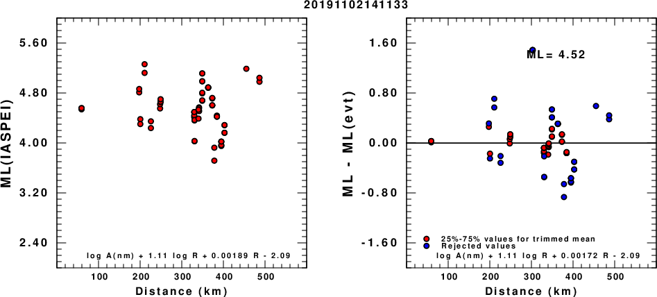
(a) ML computed using the IASPEI formula for Horizontal components; (b) ML residuals computed using a modified IASPEI formula that accounts for path specific attenuation; the values used for the trimmed mean are indicated. The ML relation used for each figure is given at the bottom of each plot.
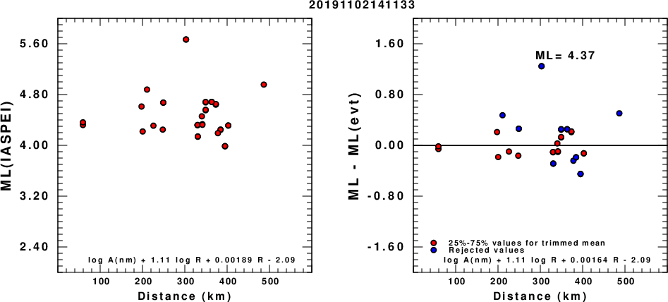
(a) ML computed using the IASPEI formula for Vertical components (research); (b) ML residuals computed using a modified IASPEI formula that accounts for path specific attenuation; the values used for the trimmed mean are indicated. The ML relation used for each figure is given at the bottom of each plot.
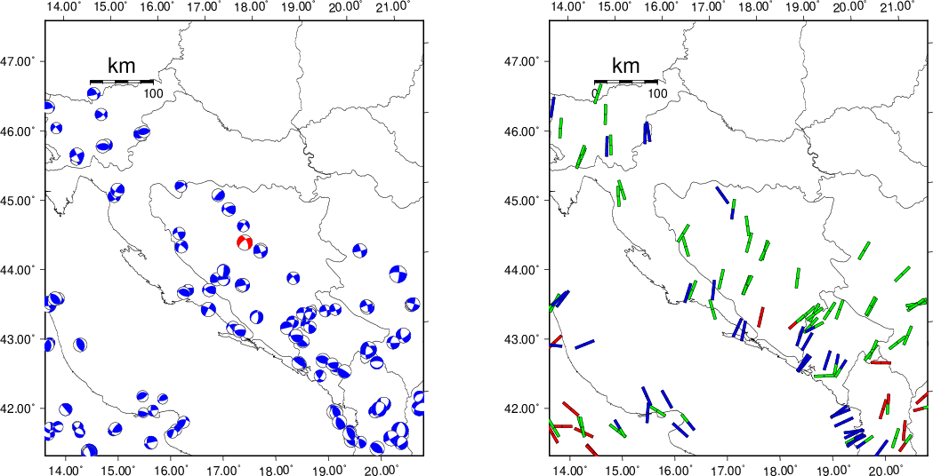 |
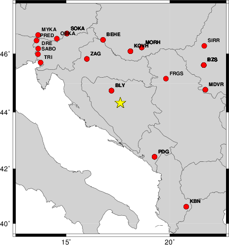
The focal mechanism was determined using broadband seismic waveforms. The location of the event and the and stations used for the waveform inversion are shown in the next figure.
|
|
|
The program wvfgrd96 was used with good traces observed at short distance to determine the focal mechanism, depth and seismic moment. This technique requires a high quality signal and well determined velocity model for the Green functions. To the extent that these are the quality data, this type of mechanism should be preferred over the radiation pattern technique which requires the separate step of defining the pressure and tension quadrants and the correct strike.
The observed and predicted traces are filtered using the following gsac commands:
cut o DIST/3.3 -30 o DIST/3.3 +70
rtr
taper w 0.1
hp c 0.02 n 3
lp c 0.06 n 3
The results of this grid search from 0.5 to 19 km depth are as follow:
           DEPTH  STK   DIP  RAKE   MW    FIT
WVFGRD96    1.0   265    45    65   4.45 0.3599
WVFGRD96    2.0   265    50    65   4.57 0.4753
WVFGRD96    3.0   115    45   110   4.64 0.5380
WVFGRD96    4.0   270    45    75   4.67 0.5394
WVFGRD96    5.0   245    55    45   4.63 0.5105
WVFGRD96    6.0   230    80    25   4.59 0.5139
WVFGRD96    7.0   230    85    20   4.61 0.5260
WVFGRD96    8.0   235    75    30   4.65 0.5396
WVFGRD96    9.0   230    65   -35   4.69 0.5576
WVFGRD96   10.0   230    65   -35   4.70 0.5727
WVFGRD96   11.0   230    65   -35   4.71 0.5850
WVFGRD96   12.0   235    70   -30   4.72 0.5949
WVFGRD96   13.0   235    70   -30   4.73 0.6025
WVFGRD96   14.0   235    70   -30   4.74 0.6080
WVFGRD96   15.0   235    70   -30   4.75 0.6116
WVFGRD96   16.0   235    65   -30   4.76 0.6142
WVFGRD96   17.0   235    65   -30   4.77 0.6155
WVFGRD96   18.0   235    65   -30   4.78 0.6158
WVFGRD96   19.0   235    65   -30   4.78 0.6152
WVFGRD96   20.0   235    65   -30   4.79 0.6139
WVFGRD96   21.0   235    65   -30   4.80 0.6117
WVFGRD96   22.0   235    65   -30   4.81 0.6092
WVFGRD96   23.0   235    65   -30   4.81 0.6057
WVFGRD96   24.0   235    65   -30   4.82 0.6013
WVFGRD96   25.0   235    60   -30   4.83 0.5969
WVFGRD96   26.0   235    60   -30   4.83 0.5920
WVFGRD96   27.0   235    60   -30   4.84 0.5860
WVFGRD96   28.0   235    60   -30   4.84 0.5793
WVFGRD96   29.0   235    60   -30   4.85 0.5717
The best solution is
WVFGRD96 18.0 235 65 -30 4.78 0.6158
The mechanism correspond to the best fit is
|
|
|
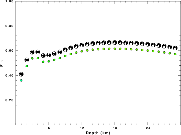
The best fit as a function of depth is given in the following figure:
|
|
|
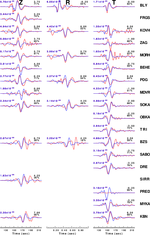
The comparison of the observed and predicted waveforms is given in the next figure. The red traces are the observed and the blue are the predicted. Each observed-predicted component is plotted to the same scale and peak amplitudes are indicated by the numbers to the left of each trace. A pair of numbers is given in black at the right of each predicted traces. The upper number it the time shift required for maximum correlation between the observed and predicted traces. This time shift is required because the synthetics are not computed at exactly the same distance as the observed and because the velocity model used in the predictions may not be perfect. A positive time shift indicates that the prediction is too fast and should be delayed to match the observed trace (shift to the right in this figure). A negative value indicates that the prediction is too slow. The lower number gives the percentage of variance reduction to characterize the individual goodness of fit (100% indicates a perfect fit).
The bandpass filter used in the processing and for the display was
cut o DIST/3.3 -30 o DIST/3.3 +70
rtr
taper w 0.1
hp c 0.02 n 3
lp c 0.06 n 3
|
|
|
|
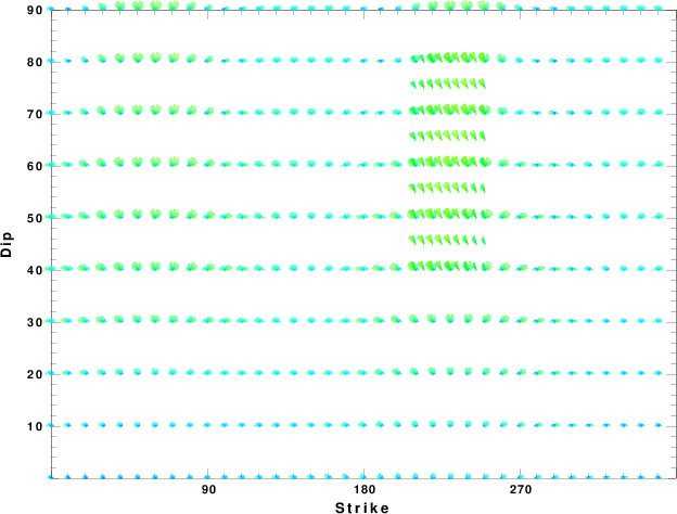
| Focal mechanism sensitivity at the preferred depth. The red color indicates a very good fit to thewavefroms. Each solution is plotted as a vector at a given value of strike and dip with the angle of the vector representing the rake angle, measured, with respect to the upward vertical (N) in the figure. |
A check on the assumed source location is possible by looking at the time shifts between the observed and predicted traces. The time shifts for waveform matching arise for several reasons:
Time_shift = A + B cos Azimuth + C Sin Azimuth
The time shifts for this inversion lead to the next figure:
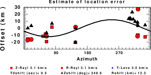
The derived shift in origin time and epicentral coordinates are given at the bottom of the figure.
Thanks also to the many seismic network operators whose dedication make this effort possible: University of Nevada Reno, University of Alaska, University of Washington, Oregon State University, University of Utah, Montana Bureas of Mines, UC Berkely, Caltech, UC San Diego, Saint Louis University, University of Memphis, Lamont Doherty Earth Observatory, the Iris stations and the Transportable Array of EarthScope.
The WUS.model used for the waveform synthetic seismograms and for the surface wave eigenfunctions and dispersion is as follows:
MODEL.01
Model after     8 iterations
ISOTROPIC
KGS
FLAT EARTH
1-D
CONSTANT VELOCITY
LINE08
LINE09
LINE10
LINE11
      H(KM)   VP(KM/S)   VS(KM/S) RHO(GM/CC)         QP         QS       ETAP       ETAS      FREFP      FREFS
     1.9000     3.4065     2.0089     2.2150  0.302E-02  0.679E-02   0.00       0.00       1.00       1.00
     6.1000     5.5445     3.2953     2.6089  0.349E-02  0.784E-02   0.00       0.00       1.00       1.00
    13.0000     6.2708     3.7396     2.7812  0.212E-02  0.476E-02   0.00       0.00       1.00       1.00
    19.0000     6.4075     3.7680     2.8223  0.111E-02  0.249E-02   0.00       0.00       1.00       1.00
     0.0000     7.9000     4.6200     3.2760  0.164E-10  0.370E-10   0.00       0.00       1.00       1.00
Here we tabulate the reasons for not using certain digital data sets
The following stations did not have a valid response files: