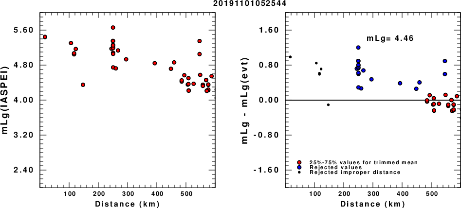
(a) mLg computed using the IASPEI formula; (b) mLg residuals ; the values used for the trimmed mean are indicated.
 USGS/SLU Moment Tensor Solution
 ENS  2019/11/01 05:25:44:3  40.47   20.75  10.0 4.7 Albania

 Stations used:
   AC.KBN AC.VLO CL.AGRP CL.MALA CL.MG03 CL.MG04 CL.MG05
   CL.MG06 CL.MG07 CL.PSAM HT.ALN HU.KOVH MN.BLY MN.BZS MN.KEK
   MN.KLV MN.PDG RO.DEV RO.GZR RO.HERR RO.MDVR RO.PUNG RO.SIRR
   SJ.BBLS

 Filtering commands used:
   cut o DIST/3.3 -30 o DIST/3.3 +70
   rtr
   taper w 0.1
   hp c 0.02 n 3
   lp c 0.06 n 3

 Best Fitting Double Couple
  Mo = 1.62e+23 dyne-cm
  Mw = 4.74
  Z  = 14 km
  Plane   Strike  Dip  Rake
   NP1      270    60    40
   NP2      157    56   143
  Principal Axes:
   Axis    Value   Plunge  Azimuth
    T   1.62e+23     48     125
    N   0.00e+00     42     301
    P  -1.62e+23      2      33

 Moment Tensor: (dyne-cm)
    Component   Value
       Mxx    -9.03e+22
       Mxy    -1.08e+23
       Mxz    -5.21e+22
       Myy    -2.57e+15
       Myz     6.21e+22
       Mzz     9.03e+22


                     --------------
                 ##------------------ P
              ####-------------------   --
             #####-------------------------
           #######---------------------------
          ########----------------------------
         #########-----------------------------
        ##########-##################-----------
        ######----########################------
       ###--------############################---
       #-----------#############################-
       ------------##############################
       -------------#############################
        -------------##############   ##########
        --------------############# T ##########
         --------------############   #########
          --------------######################
           --------------####################
             --------------################
              ---------------#############
                 ---------------#######
                     --------------


 Global CMT Convention Moment Tensor:
      R          T          P
  9.03e+22  -5.21e+22  -6.21e+22
 -5.21e+22  -9.03e+22   1.08e+23
 -6.21e+22   1.08e+23  -2.57e+15


Details of the solution is found at

http://www.eas.slu.edu/eqc/eqc_mt/MECH.NA/20191101052544/index.html
|
      STK = 270
      DIP = 60
     RAKE = 40
       MW = 4.74
       HS = 14.0
The NDK file is 20191101052544.ndk The OCA solution is Mw=4.7 STK=90 DIP=50 RAKE=28 H=9 km. The solution is described in seismoazur.jpg
The following compares this source inversion to others
 USGS/SLU Moment Tensor Solution
 ENS  2019/11/01 05:25:44:3  40.47   20.75  10.0 4.7 Albania

 Stations used:
   AC.KBN AC.VLO CL.AGRP CL.MALA CL.MG03 CL.MG04 CL.MG05
   CL.MG06 CL.MG07 CL.PSAM HT.ALN HU.KOVH MN.BLY MN.BZS MN.KEK
   MN.KLV MN.PDG RO.DEV RO.GZR RO.HERR RO.MDVR RO.PUNG RO.SIRR
   SJ.BBLS

 Filtering commands used:
   cut o DIST/3.3 -30 o DIST/3.3 +70
   rtr
   taper w 0.1
   hp c 0.02 n 3
   lp c 0.06 n 3

 Best Fitting Double Couple
  Mo = 1.62e+23 dyne-cm
  Mw = 4.74
  Z  = 14 km
  Plane   Strike  Dip  Rake
   NP1      270    60    40
   NP2      157    56   143
  Principal Axes:
   Axis    Value   Plunge  Azimuth
    T   1.62e+23     48     125
    N   0.00e+00     42     301
    P  -1.62e+23      2      33

 Moment Tensor: (dyne-cm)
    Component   Value
       Mxx    -9.03e+22
       Mxy    -1.08e+23
       Mxz    -5.21e+22
       Myy    -2.57e+15
       Myz     6.21e+22
       Mzz     9.03e+22


                     --------------
                 ##------------------ P
              ####-------------------   --
             #####-------------------------
           #######---------------------------
          ########----------------------------
         #########-----------------------------
        ##########-##################-----------
        ######----########################------
       ###--------############################---
       #-----------#############################-
       ------------##############################
       -------------#############################
        -------------##############   ##########
        --------------############# T ##########
         --------------############   #########
          --------------######################
           --------------####################
             --------------################
              ---------------#############
                 ---------------#######
                     --------------


 Global CMT Convention Moment Tensor:
      R          T          P
  9.03e+22  -5.21e+22  -6.21e+22
 -5.21e+22  -9.03e+22   1.08e+23
 -6.21e+22   1.08e+23  -2.57e+15


Details of the solution is found at

http://www.eas.slu.edu/eqc/eqc_mt/MECH.NA/20191101052544/index.html
|
(a) mLg computed using the IASPEI formula; (b) mLg residuals ; the values used for the trimmed mean are indicated.
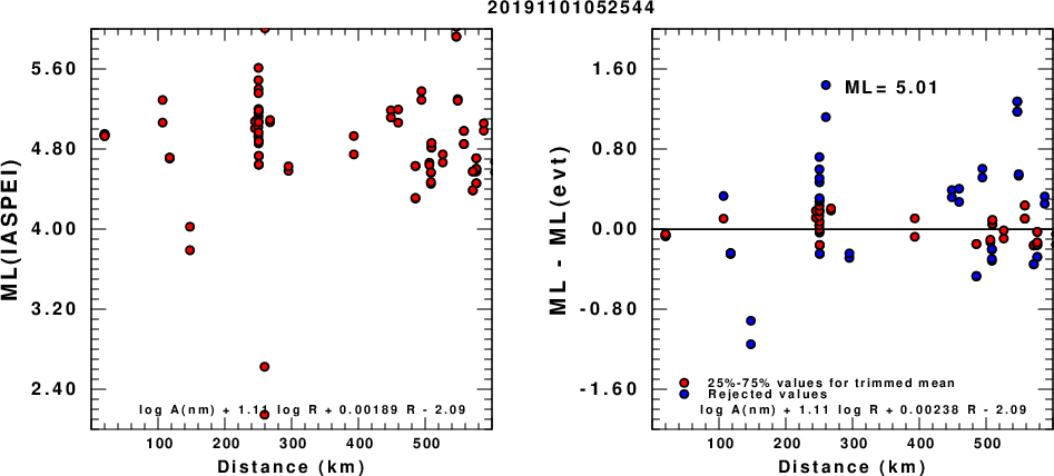
(a) ML computed using the IASPEI formula for Horizontal components; (b) ML residuals computed using a modified IASPEI formula that accounts for path specific attenuation; the values used for the trimmed mean are indicated. The ML relation used for each figure is given at the bottom of each plot.
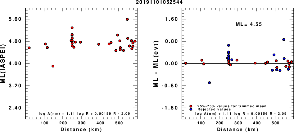
(a) ML computed using the IASPEI formula for Vertical components (research); (b) ML residuals computed using a modified IASPEI formula that accounts for path specific attenuation; the values used for the trimmed mean are indicated. The ML relation used for each figure is given at the bottom of each plot.
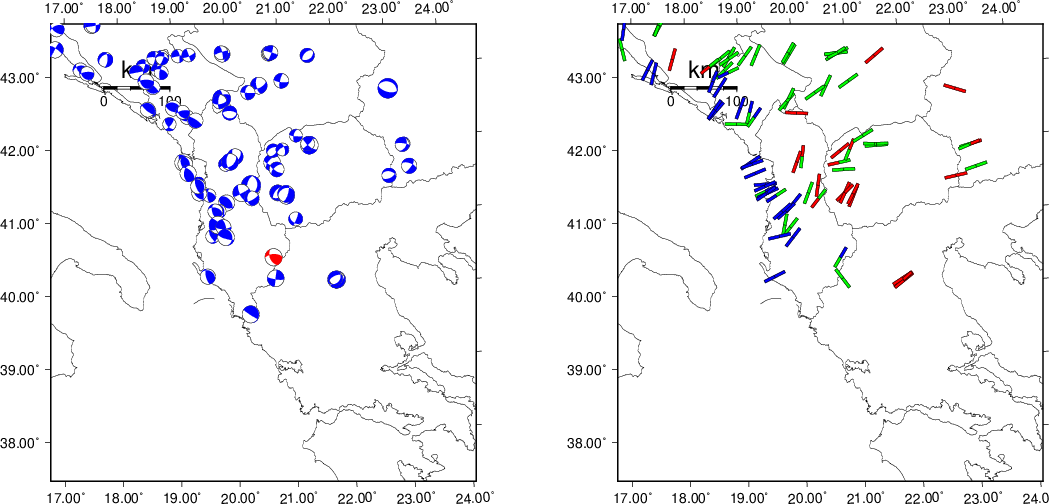 |
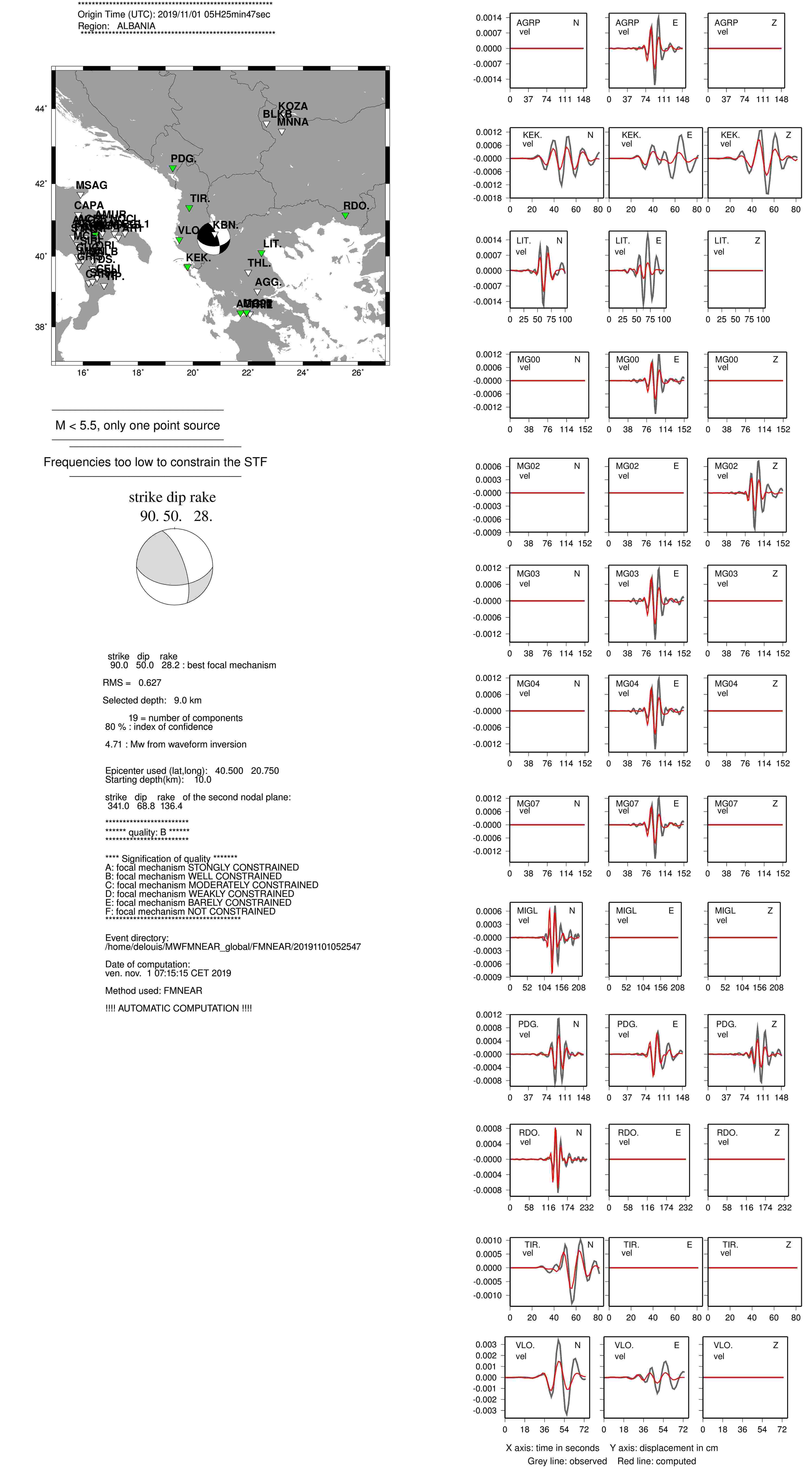
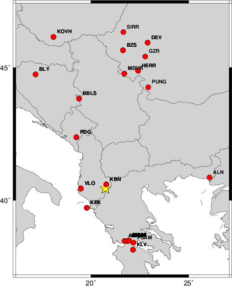
The focal mechanism was determined using broadband seismic waveforms. The location of the event and the and stations used for the waveform inversion are shown in the next figure.
|
|
|
The program wvfgrd96 was used with good traces observed at short distance to determine the focal mechanism, depth and seismic moment. This technique requires a high quality signal and well determined velocity model for the Green functions. To the extent that these are the quality data, this type of mechanism should be preferred over the radiation pattern technique which requires the separate step of defining the pressure and tension quadrants and the correct strike.
The observed and predicted traces are filtered using the following gsac commands:
cut o DIST/3.3 -30 o DIST/3.3 +70
rtr
taper w 0.1
hp c 0.02 n 3
lp c 0.06 n 3
The results of this grid search from 0.5 to 19 km depth are as follow:
           DEPTH  STK   DIP  RAKE   MW    FIT
WVFGRD96    1.0   180    60    40   4.40 0.3148
WVFGRD96    2.0   180    60    35   4.50 0.3957
WVFGRD96    3.0   185    75    50   4.57 0.4067
WVFGRD96    4.0    -5    90   -50   4.60 0.4449
WVFGRD96    5.0     0    90   -50   4.63 0.4751
WVFGRD96    6.0     0    90   -45   4.63 0.4974
WVFGRD96    7.0   180    90    40   4.64 0.5119
WVFGRD96    8.0   180    90    45   4.69 0.5221
WVFGRD96    9.0   210    65    70   4.77 0.5361
WVFGRD96   10.0   270    65    45   4.71 0.5515
WVFGRD96   11.0   270    65    45   4.72 0.5672
WVFGRD96   12.0   270    65    40   4.72 0.5766
WVFGRD96   13.0   270    65    40   4.73 0.5824
WVFGRD96   14.0   270    60    40   4.74 0.5842
WVFGRD96   15.0   270    60    40   4.75 0.5831
WVFGRD96   16.0   270    60    35   4.75 0.5805
WVFGRD96   17.0   265    65    35   4.76 0.5762
WVFGRD96   18.0   265    65    35   4.76 0.5710
WVFGRD96   19.0   265    65    35   4.77 0.5645
WVFGRD96   20.0   265    65    30   4.78 0.5572
WVFGRD96   21.0   265    65    30   4.79 0.5492
WVFGRD96   22.0   265    65    30   4.79 0.5413
WVFGRD96   23.0   265    65    30   4.80 0.5323
WVFGRD96   24.0   265    65    30   4.80 0.5229
WVFGRD96   25.0   265    65    30   4.81 0.5138
WVFGRD96   26.0   265    65    30   4.81 0.5039
WVFGRD96   27.0   265    65    30   4.82 0.4938
WVFGRD96   28.0   265    65    30   4.82 0.4834
WVFGRD96   29.0   265    65    30   4.82 0.4730
The best solution is
WVFGRD96 14.0 270 60 40 4.74 0.5842
The mechanism correspond to the best fit is
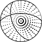
|
|
|
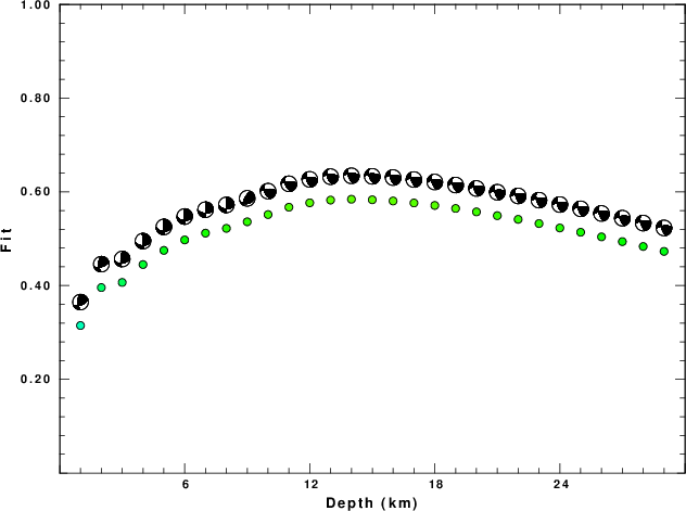
The best fit as a function of depth is given in the following figure:
|
|
|
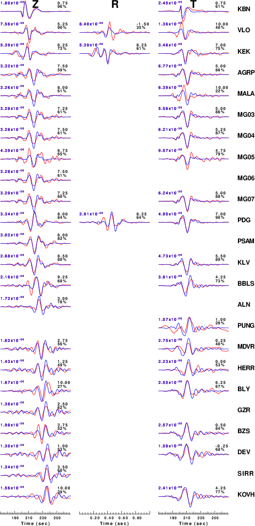
The comparison of the observed and predicted waveforms is given in the next figure. The red traces are the observed and the blue are the predicted. Each observed-predicted component is plotted to the same scale and peak amplitudes are indicated by the numbers to the left of each trace. A pair of numbers is given in black at the right of each predicted traces. The upper number it the time shift required for maximum correlation between the observed and predicted traces. This time shift is required because the synthetics are not computed at exactly the same distance as the observed and because the velocity model used in the predictions may not be perfect. A positive time shift indicates that the prediction is too fast and should be delayed to match the observed trace (shift to the right in this figure). A negative value indicates that the prediction is too slow. The lower number gives the percentage of variance reduction to characterize the individual goodness of fit (100% indicates a perfect fit).
The bandpass filter used in the processing and for the display was
cut o DIST/3.3 -30 o DIST/3.3 +70
rtr
taper w 0.1
hp c 0.02 n 3
lp c 0.06 n 3
|
|
|
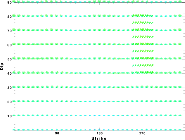
|
| Focal mechanism sensitivity at the preferred depth. The red color indicates a very good fit to thewavefroms. Each solution is plotted as a vector at a given value of strike and dip with the angle of the vector representing the rake angle, measured, with respect to the upward vertical (N) in the figure. |
A check on the assumed source location is possible by looking at the time shifts between the observed and predicted traces. The time shifts for waveform matching arise for several reasons:
Time_shift = A + B cos Azimuth + C Sin Azimuth
The time shifts for this inversion lead to the next figure:
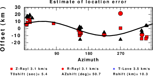
The derived shift in origin time and epicentral coordinates are given at the bottom of the figure.
Thanks also to the many seismic network operators whose dedication make this effort possible: University of Nevada Reno, University of Alaska, University of Washington, Oregon State University, University of Utah, Montana Bureas of Mines, UC Berkely, Caltech, UC San Diego, Saint Louis University, University of Memphis, Lamont Doherty Earth Observatory, the Iris stations and the Transportable Array of EarthScope.
The WUS.model used for the waveform synthetic seismograms and for the surface wave eigenfunctions and dispersion is as follows:
MODEL.01
Model after     8 iterations
ISOTROPIC
KGS
FLAT EARTH
1-D
CONSTANT VELOCITY
LINE08
LINE09
LINE10
LINE11
      H(KM)   VP(KM/S)   VS(KM/S) RHO(GM/CC)         QP         QS       ETAP       ETAS      FREFP      FREFS
     1.9000     3.4065     2.0089     2.2150  0.302E-02  0.679E-02   0.00       0.00       1.00       1.00
     6.1000     5.5445     3.2953     2.6089  0.349E-02  0.784E-02   0.00       0.00       1.00       1.00
    13.0000     6.2708     3.7396     2.7812  0.212E-02  0.476E-02   0.00       0.00       1.00       1.00
    19.0000     6.4075     3.7680     2.8223  0.111E-02  0.249E-02   0.00       0.00       1.00       1.00
     0.0000     7.9000     4.6200     3.2760  0.164E-10  0.370E-10   0.00       0.00       1.00       1.00
Here we tabulate the reasons for not using certain digital data sets
The following stations did not have a valid response files: