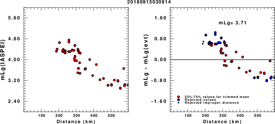
(a) mLg computed using the IASPEI formula; (b) mLg residuals ; the values used for the trimmed mean are indicated.
 USGS/SLU Moment Tensor Solution
 ENS  2018/09/15 03:09:14:3  43.83   15.80   2.0 4.2 Croatia

 Stations used:
   CZ.JAVC HU.BEHE HU.BUD HU.CSKK HU.EGYH HU.KOVH HU.MPLH
   HU.TIH NI.PALA OE.MYKA OE.OBKA OE.SOKA SJ.BBLS SL.BOJS
   SL.CADS SL.CEY SL.CRES SL.CRNS SL.GBAS SL.GBRS SL.GCIS
   SL.GORS SL.GROS SL.KOGS SL.LJU SL.MOZS SL.PERS SL.ROBS
   SL.SKDS SL.VISS SL.VOJS

 Filtering commands used:
   cut o DIST/3.3 -30 o DIST/3.3 +50
   rtr
   taper w 0.1
   hp c 0.02 n 3
   lp c 0.06 n 3

 Best Fitting Double Couple
  Mo = 1.91e+22 dyne-cm
  Mw = 4.12
  Z  = 14 km
  Plane   Strike  Dip  Rake
   NP1      161    72   154
   NP2      260    65    20
  Principal Axes:
   Axis    Value   Plunge  Azimuth
    T   1.91e+22     31     119
    N   0.00e+00     58     309
    P  -1.91e+22      5     212

 Moment Tensor: (dyne-cm)
    Component   Value
       Mxx    -1.04e+22
       Mxy    -1.44e+22
       Mxz    -2.81e+21
       Myy     5.40e+21
       Myz     8.18e+21
       Mzz     4.99e+21


                     --------------
                 ####------------------
              #######---------------------
             ########----------------------
           ##########------------------------
          ###########-------------------------
         ############--------------------------
        ##############------#############-------
        ############--#########################-
       #########------###########################
       ######----------##########################
       ###-------------##########################
       #----------------#########################
        -----------------##############   ######
        ------------------############# T ######
         -----------------#############   #####
          -----------------###################
           -----------------#################
             -----------------#############
              ---   -----------###########
                  P ------------#######
                     -------------#


 Global CMT Convention Moment Tensor:
      R          T          P
  4.99e+21  -2.81e+21  -8.18e+21
 -2.81e+21  -1.04e+22   1.44e+22
 -8.18e+21   1.44e+22   5.40e+21


Details of the solution is found at

http://www.eas.slu.edu/eqc/eqc_mt/MECH.NA/20180915030914/index.html
|
      STK = 260
      DIP = 65
     RAKE = 20
       MW = 4.12
       HS = 14.0
The NDK file is 20180915030914.ndk The waveform inversion is preferred.
The following compares this source inversion to others
 USGS/SLU Moment Tensor Solution
 ENS  2018/09/15 03:09:14:3  43.83   15.80   2.0 4.2 Croatia

 Stations used:
   CZ.JAVC HU.BEHE HU.BUD HU.CSKK HU.EGYH HU.KOVH HU.MPLH
   HU.TIH NI.PALA OE.MYKA OE.OBKA OE.SOKA SJ.BBLS SL.BOJS
   SL.CADS SL.CEY SL.CRES SL.CRNS SL.GBAS SL.GBRS SL.GCIS
   SL.GORS SL.GROS SL.KOGS SL.LJU SL.MOZS SL.PERS SL.ROBS
   SL.SKDS SL.VISS SL.VOJS

 Filtering commands used:
   cut o DIST/3.3 -30 o DIST/3.3 +50
   rtr
   taper w 0.1
   hp c 0.02 n 3
   lp c 0.06 n 3

 Best Fitting Double Couple
  Mo = 1.91e+22 dyne-cm
  Mw = 4.12
  Z  = 14 km
  Plane   Strike  Dip  Rake
   NP1      161    72   154
   NP2      260    65    20
  Principal Axes:
   Axis    Value   Plunge  Azimuth
    T   1.91e+22     31     119
    N   0.00e+00     58     309
    P  -1.91e+22      5     212

 Moment Tensor: (dyne-cm)
    Component   Value
       Mxx    -1.04e+22
       Mxy    -1.44e+22
       Mxz    -2.81e+21
       Myy     5.40e+21
       Myz     8.18e+21
       Mzz     4.99e+21


                     --------------
                 ####------------------
              #######---------------------
             ########----------------------
           ##########------------------------
          ###########-------------------------
         ############--------------------------
        ##############------#############-------
        ############--#########################-
       #########------###########################
       ######----------##########################
       ###-------------##########################
       #----------------#########################
        -----------------##############   ######
        ------------------############# T ######
         -----------------#############   #####
          -----------------###################
           -----------------#################
             -----------------#############
              ---   -----------###########
                  P ------------#######
                     -------------#


 Global CMT Convention Moment Tensor:
      R          T          P
  4.99e+21  -2.81e+21  -8.18e+21
 -2.81e+21  -1.04e+22   1.44e+22
 -8.18e+21   1.44e+22   5.40e+21


Details of the solution is found at

http://www.eas.slu.edu/eqc/eqc_mt/MECH.NA/20180915030914/index.html
|
(a) mLg computed using the IASPEI formula; (b) mLg residuals ; the values used for the trimmed mean are indicated.
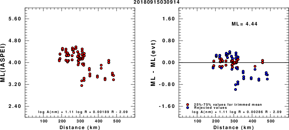
(a) ML computed using the IASPEI formula for Horizontal components; (b) ML residuals computed using a modified IASPEI formula that accounts for path specific attenuation; the values used for the trimmed mean are indicated. The ML relation used for each figure is given at the bottom of each plot.
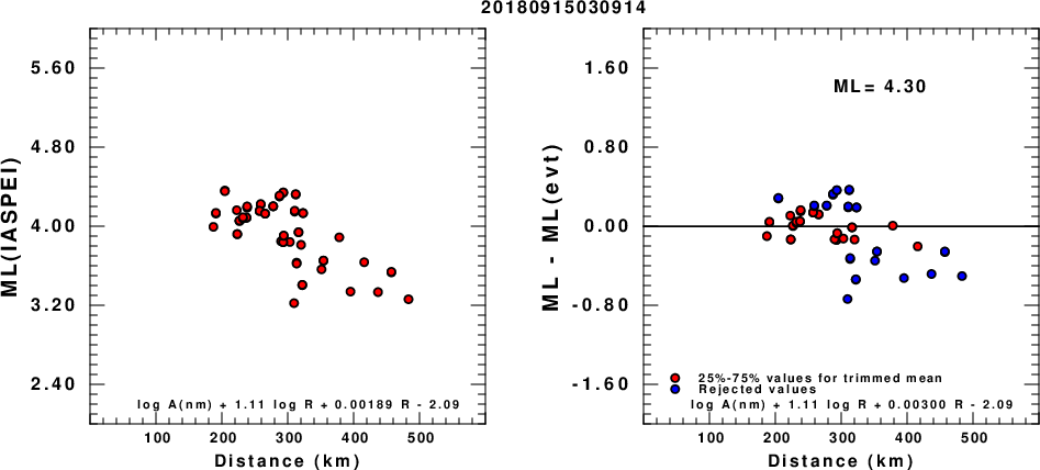
(a) ML computed using the IASPEI formula for Vertical components (research); (b) ML residuals computed using a modified IASPEI formula that accounts for path specific attenuation; the values used for the trimmed mean are indicated. The ML relation used for each figure is given at the bottom of each plot.
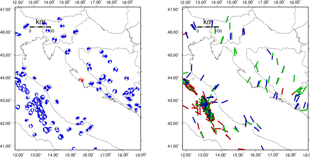 |
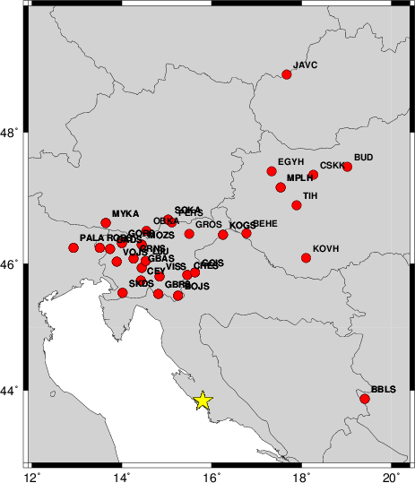
The focal mechanism was determined using broadband seismic waveforms. The location of the event and the and stations used for the waveform inversion are shown in the next figure.
|
|
|
The program wvfgrd96 was used with good traces observed at short distance to determine the focal mechanism, depth and seismic moment. This technique requires a high quality signal and well determined velocity model for the Green functions. To the extent that these are the quality data, this type of mechanism should be preferred over the radiation pattern technique which requires the separate step of defining the pressure and tension quadrants and the correct strike.
The observed and predicted traces are filtered using the following gsac commands:
cut o DIST/3.3 -30 o DIST/3.3 +50
rtr
taper w 0.1
hp c 0.02 n 3
lp c 0.06 n 3
The results of this grid search from 0.5 to 19 km depth are as follow:
           DEPTH  STK   DIP  RAKE   MW    FIT
WVFGRD96    1.0   250    70   -35   3.85 0.3044
WVFGRD96    2.0   250    65   -30   3.92 0.3603
WVFGRD96    3.0   250    60   -30   3.96 0.3814
WVFGRD96    4.0   255    65   -20   3.96 0.3960
WVFGRD96    5.0   255    70   -20   3.97 0.4082
WVFGRD96    6.0   260    70    15   3.99 0.4226
WVFGRD96    7.0   260    70    15   4.01 0.4376
WVFGRD96    8.0   260    70    20   4.04 0.4490
WVFGRD96    9.0   260    70    20   4.05 0.4580
WVFGRD96   10.0   260    70    20   4.07 0.4645
WVFGRD96   11.0   260    65    20   4.09 0.4689
WVFGRD96   12.0   260    65    20   4.10 0.4717
WVFGRD96   13.0   260    65    20   4.11 0.4732
WVFGRD96   14.0   260    65    20   4.12 0.4734
WVFGRD96   15.0   260    65    15   4.13 0.4730
WVFGRD96   16.0   260    65    15   4.14 0.4717
WVFGRD96   17.0   260    65    15   4.15 0.4695
WVFGRD96   18.0   260    65    15   4.16 0.4664
WVFGRD96   19.0   260    65    15   4.17 0.4625
WVFGRD96   20.0   260    65    15   4.18 0.4585
WVFGRD96   21.0   260    65    15   4.19 0.4534
WVFGRD96   22.0   260    65    15   4.19 0.4479
WVFGRD96   23.0   260    65    15   4.20 0.4417
WVFGRD96   24.0   260    65    15   4.21 0.4349
WVFGRD96   25.0   260    65    15   4.22 0.4277
WVFGRD96   26.0   260    65    15   4.23 0.4203
WVFGRD96   27.0   260    65    15   4.23 0.4124
WVFGRD96   28.0   260    65    15   4.24 0.4042
WVFGRD96   29.0   260    65    15   4.25 0.3954
The best solution is
WVFGRD96 14.0 260 65 20 4.12 0.4734
The mechanism correspond to the best fit is
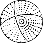
|
|
|
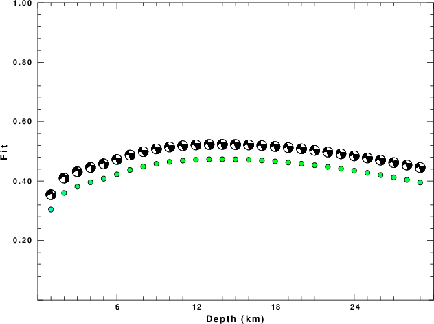
The best fit as a function of depth is given in the following figure:
|
|
|
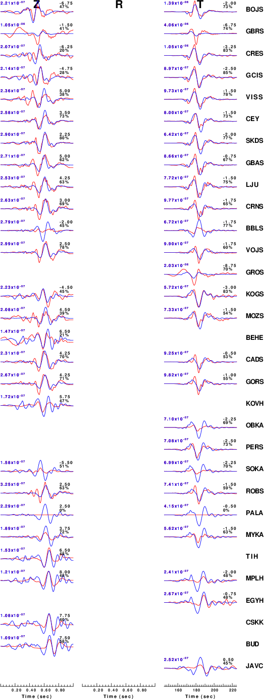
The comparison of the observed and predicted waveforms is given in the next figure. The red traces are the observed and the blue are the predicted. Each observed-predicted component is plotted to the same scale and peak amplitudes are indicated by the numbers to the left of each trace. A pair of numbers is given in black at the right of each predicted traces. The upper number it the time shift required for maximum correlation between the observed and predicted traces. This time shift is required because the synthetics are not computed at exactly the same distance as the observed and because the velocity model used in the predictions may not be perfect. A positive time shift indicates that the prediction is too fast and should be delayed to match the observed trace (shift to the right in this figure). A negative value indicates that the prediction is too slow. The lower number gives the percentage of variance reduction to characterize the individual goodness of fit (100% indicates a perfect fit).
The bandpass filter used in the processing and for the display was
cut o DIST/3.3 -30 o DIST/3.3 +50
rtr
taper w 0.1
hp c 0.02 n 3
lp c 0.06 n 3
|
|
|
|
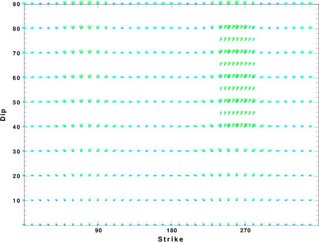
| Focal mechanism sensitivity at the preferred depth. The red color indicates a very good fit to thewavefroms. Each solution is plotted as a vector at a given value of strike and dip with the angle of the vector representing the rake angle, measured, with respect to the upward vertical (N) in the figure. |
A check on the assumed source location is possible by looking at the time shifts between the observed and predicted traces. The time shifts for waveform matching arise for several reasons:
Time_shift = A + B cos Azimuth + C Sin Azimuth
The time shifts for this inversion lead to the next figure:
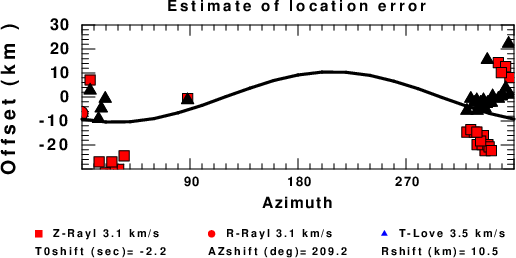
The derived shift in origin time and epicentral coordinates are given at the bottom of the figure.
Thanks also to the many seismic network operators whose dedication make this effort possible: University of Nevada Reno, University of Alaska, University of Washington, Oregon State University, University of Utah, Montana Bureas of Mines, UC Berkely, Caltech, UC San Diego, Saint Louis University, University of Memphis, Lamont Doherty Earth Observatory, the Iris stations and the Transportable Array of EarthScope.
The WUS.model used for the waveform synthetic seismograms and for the surface wave eigenfunctions and dispersion is as follows:
MODEL.01
Model after     8 iterations
ISOTROPIC
KGS
FLAT EARTH
1-D
CONSTANT VELOCITY
LINE08
LINE09
LINE10
LINE11
      H(KM)   VP(KM/S)   VS(KM/S) RHO(GM/CC)         QP         QS       ETAP       ETAS      FREFP      FREFS
     1.9000     3.4065     2.0089     2.2150  0.302E-02  0.679E-02   0.00       0.00       1.00       1.00
     6.1000     5.5445     3.2953     2.6089  0.349E-02  0.784E-02   0.00       0.00       1.00       1.00
    13.0000     6.2708     3.7396     2.7812  0.212E-02  0.476E-02   0.00       0.00       1.00       1.00
    19.0000     6.4075     3.7680     2.8223  0.111E-02  0.249E-02   0.00       0.00       1.00       1.00
     0.0000     7.9000     4.6200     3.2760  0.164E-10  0.370E-10   0.00       0.00       1.00       1.00
Here we tabulate the reasons for not using certain digital data sets
The following stations did not have a valid response files: