Location

Location ANSS

2018/07/17 13:05:08 41.09 19.69 10.0 4.6 Albania

Focal Mechanism

USGS/SLU Moment Tensor Solution ENS 2018/07/17 13:05:08:4 41.09 19.69 10.0 4.6 Albania Stations used: CL.MALA CL.MG05 CL.MG07 HL.EVR HL.JAN HL.KLV HL.KYMI HL.LIA HL.NEO HL.NVR HL.PLG HL.SMTH HL.THL HL.VLS HL.VLY HP.AMT HP.ANX HP.GUR HP.PVO HT.AGG HT.ALN HT.AOS2 HT.IGT HT.KAVA HT.KOKK HT.KRND HT.NEST HT.OUR HT.SIGR HT.SOH HT.THAS HU.KOVH HU.MORH ME.KOME RO.BZS RO.GZR SJ.FRGS Filtering commands used: cut o DIST/3.3 -30 o DIST/3.3 +70 rtr taper w 0.1 hp c 0.03 n 3 lp c 0.08 n 3 Best Fitting Double Couple Mo = 2.11e+22 dyne-cm Mw = 4.15 Z = 27 km Plane Strike Dip Rake NP1 152 73 132 NP2 260 45 25 Principal Axes: Axis Value Plunge Azimuth T 2.11e+22 45 104 N 0.00e+00 40 317 P -2.11e+22 17 212 Moment Tensor: (dyne-cm) Component Value Mxx -1.33e+22 Mxy -1.12e+22 Mxz 2.35e+21 Myy 4.36e+21 Myz 1.33e+22 Mzz 8.93e+21 -------------- #--------------------- ####------------------------ #####------------------------- ########-------------------------- #########---#################------- #########--#######################---- #######-----##########################-- #####--------########################### ####-----------########################### ###-------------########################## ##--------------############## ######### #----------------############# T ######### ------------------########### ######## -------------------##################### -------------------################### -------------------################# --------------------############## ---- ------------########### --- P --------------######## -----------------## -------------- Global CMT Convention Moment Tensor: R T P 8.93e+21 2.35e+21 -1.33e+22 2.35e+21 -1.33e+22 1.12e+22 -1.33e+22 1.12e+22 4.36e+21 Details of the solution is found at http://www.eas.slu.edu/eqc/eqc_mt/MECH.NA/20180717130508/index.html

Preferred Solution

The preferred solution from an analysis of the surface-wave spectral amplitude radiation pattern, waveform inversion and first motion observations is

      STK = 260
      DIP = 45
     RAKE = 25
       MW = 4.15
       HS = 27.0

The NDK file is 20180717130508.ndk The waveform inversion is preferred.

Moment Tensor Comparison

The following compares this source inversion to others

SLU

USGS/SLU Moment Tensor Solution ENS 2018/07/17 13:05:08:4 41.09 19.69 10.0 4.6 Albania Stations used: CL.MALA CL.MG05 CL.MG07 HL.EVR HL.JAN HL.KLV HL.KYMI HL.LIA HL.NEO HL.NVR HL.PLG HL.SMTH HL.THL HL.VLS HL.VLY HP.AMT HP.ANX HP.GUR HP.PVO HT.AGG HT.ALN HT.AOS2 HT.IGT HT.KAVA HT.KOKK HT.KRND HT.NEST HT.OUR HT.SIGR HT.SOH HT.THAS HU.KOVH HU.MORH ME.KOME RO.BZS RO.GZR SJ.FRGS Filtering commands used: cut o DIST/3.3 -30 o DIST/3.3 +70 rtr taper w 0.1 hp c 0.03 n 3 lp c 0.08 n 3 Best Fitting Double Couple Mo = 2.11e+22 dyne-cm Mw = 4.15 Z = 27 km Plane Strike Dip Rake NP1 152 73 132 NP2 260 45 25 Principal Axes: Axis Value Plunge Azimuth T 2.11e+22 45 104 N 0.00e+00 40 317 P -2.11e+22 17 212 Moment Tensor: (dyne-cm) Component Value Mxx -1.33e+22 Mxy -1.12e+22 Mxz 2.35e+21 Myy 4.36e+21 Myz 1.33e+22 Mzz 8.93e+21 -------------- #--------------------- ####------------------------ #####------------------------- ########-------------------------- #########---#################------- #########--#######################---- #######-----##########################-- #####--------########################### ####-----------########################### ###-------------########################## ##--------------############## ######### #----------------############# T ######### ------------------########### ######## -------------------##################### -------------------################### -------------------################# --------------------############## ---- ------------########### --- P --------------######## -----------------## -------------- Global CMT Convention Moment Tensor: R T P 8.93e+21 2.35e+21 -1.33e+22 2.35e+21 -1.33e+22 1.12e+22 -1.33e+22 1.12e+22 4.36e+21 Details of the solution is found at http://www.eas.slu.edu/eqc/eqc_mt/MECH.NA/20180717130508/index.html

Magnitudes

ML Magnitude

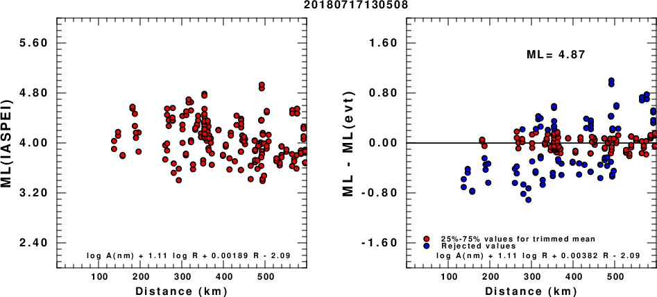
(a) ML computed using the IASPEI formula for Horizontal components; (b) ML residuals computed using a modified IASPEI formula that accounts for path specific attenuation; the values used for the trimmed mean are indicated. The ML relation used for each figure is given at the bottom of each plot.

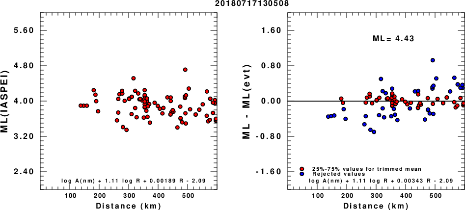
(a) ML computed using the IASPEI formula for Vertical components (research); (b) ML residuals computed using a modified IASPEI formula that accounts for path specific attenuation; the values used for the trimmed mean are indicated. The ML relation used for each figure is given at the bottom of each plot.

Context

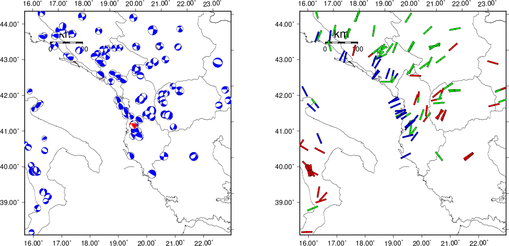
The next figure presents the focal mechanism for this earthquake (red) in the context of other events (blue) in the SLU Moment Tensor Catalog which are within ± 0.5 degrees of the new event. This comparison is shown in the left panel of the figure. The right panel shows the inferred direction of maximum compressive stress and the type of faulting (green is strike-slip, red is normal, blue is thrust; oblique is shown by a combination of colors).

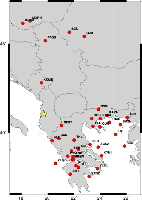
Waveform Inversion

The focal mechanism was determined using broadband seismic waveforms. The location of the event and the and stations used for the waveform inversion are shown in the next figure.

Location of broadband stations used for waveform inversion

The program wvfgrd96 was used with good traces observed at short distance to determine the focal mechanism, depth and seismic moment. This technique requires a high quality signal and well determined velocity model for the Green functions. To the extent that these are the quality data, this type of mechanism should be preferred over the radiation pattern technique which requires the separate step of defining the pressure and tension quadrants and the correct strike.

The observed and predicted traces are filtered using the following gsac commands:

cut o DIST/3.3 -30 o DIST/3.3 +70
rtr
taper w 0.1
hp c 0.03 n 3 
lp c 0.08 n 3

The results of this grid search from 0.5 to 19 km depth are as follow:

           DEPTH  STK   DIP  RAKE   MW    FIT
WVFGRD96    1.0   185    40    80   3.57 0.1284
WVFGRD96    2.0   190    45   -95   3.68 0.1660
WVFGRD96    3.0   200    40   -85   3.76 0.1882
WVFGRD96    4.0    10    50  -100   3.78 0.1779
WVFGRD96    5.0   320    60   -20   3.68 0.1771
WVFGRD96    6.0   320    65   -25   3.71 0.1868
WVFGRD96    7.0   320    65   -20   3.73 0.1965
WVFGRD96    8.0   315    60   -30   3.79 0.2046
WVFGRD96    9.0   295    55   -20   3.84 0.2129
WVFGRD96   10.0   255    40    15   3.87 0.2224
WVFGRD96   11.0   255    40    15   3.89 0.2342
WVFGRD96   12.0   255    45    20   3.90 0.2458
WVFGRD96   13.0   255    50    25   3.92 0.2591
WVFGRD96   14.0   255    50    25   3.94 0.2733
WVFGRD96   15.0   255    50    25   3.96 0.2869
WVFGRD96   16.0   255    55    25   3.97 0.2999
WVFGRD96   17.0   255    55    25   3.99 0.3118
WVFGRD96   18.0   255    55    25   4.01 0.3226
WVFGRD96   19.0   255    55    25   4.02 0.3326
WVFGRD96   20.0   255    55    25   4.04 0.3414
WVFGRD96   21.0   255    50    25   4.06 0.3485
WVFGRD96   22.0   255    50    25   4.08 0.3550
WVFGRD96   23.0   255    50    25   4.09 0.3598
WVFGRD96   24.0   255    50    25   4.10 0.3636
WVFGRD96   25.0   255    50    20   4.12 0.3663
WVFGRD96   26.0   260    45    25   4.14 0.3683
WVFGRD96   27.0   260    45    25   4.15 0.3692
WVFGRD96   28.0   260    45    25   4.16 0.3691
WVFGRD96   29.0   260    45    25   4.17 0.3682
WVFGRD96   30.0   260    40    20   4.19 0.3663
WVFGRD96   31.0   260    40    20   4.20 0.3647
WVFGRD96   32.0   260    40    20   4.20 0.3621
WVFGRD96   33.0   260    40    20   4.21 0.3597
WVFGRD96   34.0   260    40    20   4.22 0.3566
WVFGRD96   35.0   260    40    20   4.23 0.3531
WVFGRD96   36.0   260    40    20   4.24 0.3495
WVFGRD96   37.0   260    40    15   4.24 0.3454
WVFGRD96   38.0   260    40    15   4.25 0.3408
WVFGRD96   39.0   260    40    20   4.26 0.3353
WVFGRD96   40.0   295    15    65   4.42 0.3305
WVFGRD96   41.0   295    15    65   4.43 0.3256
WVFGRD96   42.0   285    20    55   4.43 0.3199
WVFGRD96   43.0   285    20    55   4.44 0.3138
WVFGRD96   44.0   285    20    55   4.45 0.3072
WVFGRD96   45.0   285    20    60   4.46 0.3006
WVFGRD96   46.0   285    20    60   4.47 0.2938
WVFGRD96   47.0   280    20    55   4.48 0.2867
WVFGRD96   48.0   280    20    55   4.49 0.2794
WVFGRD96   49.0   275    25    50   4.48 0.2719

The best solution is

WVFGRD96   27.0   260    45    25   4.15 0.3692

The mechanism correspond to the best fit is

Figure 1. Waveform inversion focal mechanism

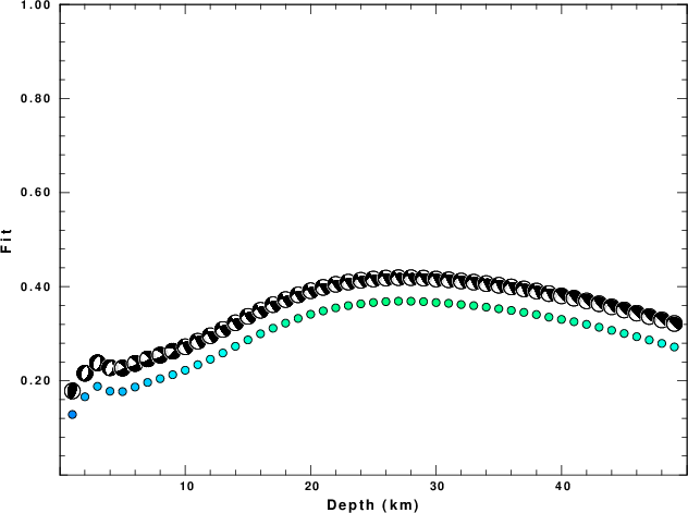
The best fit as a function of depth is given in the following figure:

Figure 2. Depth sensitivity for waveform mechanism

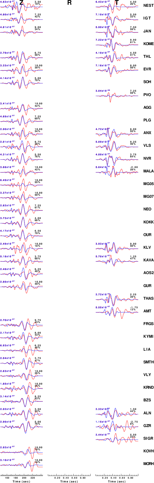
The comparison of the observed and predicted waveforms is given in the next figure. The red traces are the observed and the blue are the predicted. Each observed-predicted component is plotted to the same scale and peak amplitudes are indicated by the numbers to the left of each trace. A pair of numbers is given in black at the right of each predicted traces. The upper number it the time shift required for maximum correlation between the observed and predicted traces. This time shift is required because the synthetics are not computed at exactly the same distance as the observed and because the velocity model used in the predictions may not be perfect. A positive time shift indicates that the prediction is too fast and should be delayed to match the observed trace (shift to the right in this figure). A negative value indicates that the prediction is too slow. The lower number gives the percentage of variance reduction to characterize the individual goodness of fit (100% indicates a perfect fit).

The bandpass filter used in the processing and for the display was

cut o DIST/3.3 -30 o DIST/3.3 +70
rtr
taper w 0.1
hp c 0.03 n 3 
lp c 0.08 n 3

Figure 3. Waveform comparison for selected depth

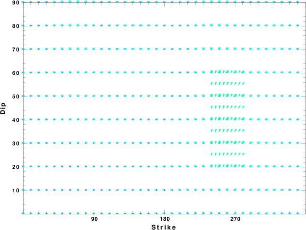
Focal mechanism sensitivity at the preferred depth. The red color indicates a very good fit to thewavefroms. Each solution is plotted as a vector at a given value of strike and dip with the angle of the vector representing the rake angle, measured, with respect to the upward vertical (N) in the figure.

A check on the assumed source location is possible by looking at the time shifts between the observed and predicted traces. The time shifts for waveform matching arise for several reasons:

The origin time and epicentral distance are incorrect
The velocity model used for the inversion is incorrect
The velocity model used to define the P-arrival time is not the same as the velocity model used for the waveform inversion (assuming that the initial trace alignment is based on the P arrival time)

Assuming only a mislocation, the time shifts are fit to a functional form:

 Time_shift = A + B cos Azimuth + C Sin Azimuth

The time shifts for this inversion lead to the next figure:

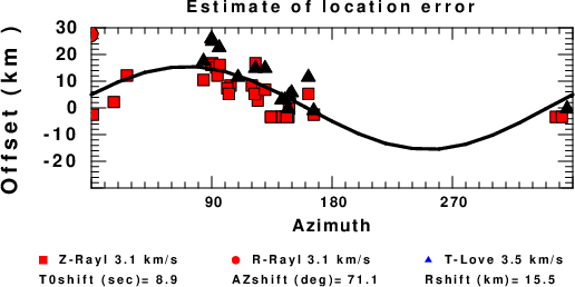
The derived shift in origin time and epicentral coordinates are given at the bottom of the figure.

Discussion

Acknowledgements

Thanks also to the many seismic network operators whose dedication make this effort possible: University of Nevada Reno, University of Alaska, University of Washington, Oregon State University, University of Utah, Montana Bureas of Mines, UC Berkely, Caltech, UC San Diego, Saint Louis University, University of Memphis, Lamont Doherty Earth Observatory, the Iris stations and the Transportable Array of EarthScope.

Velocity Model

The WUS.model used for the waveform synthetic seismograms and for the surface wave eigenfunctions and dispersion is as follows:

MODEL.01
Model after     8 iterations
ISOTROPIC
KGS
FLAT EARTH
1-D
CONSTANT VELOCITY
LINE08
LINE09
LINE10
LINE11
      H(KM)   VP(KM/S)   VS(KM/S) RHO(GM/CC)         QP         QS       ETAP       ETAS      FREFP      FREFS
     1.9000     3.4065     2.0089     2.2150  0.302E-02  0.679E-02   0.00       0.00       1.00       1.00    
     6.1000     5.5445     3.2953     2.6089  0.349E-02  0.784E-02   0.00       0.00       1.00       1.00    
    13.0000     6.2708     3.7396     2.7812  0.212E-02  0.476E-02   0.00       0.00       1.00       1.00    
    19.0000     6.4075     3.7680     2.8223  0.111E-02  0.249E-02   0.00       0.00       1.00       1.00    
     0.0000     7.9000     4.6200     3.2760  0.164E-10  0.370E-10   0.00       0.00       1.00       1.00

Quality Control

Here we tabulate the reasons for not using certain digital data sets

The following stations did not have a valid response files:

Last Changed Wed Jul 18 06:15:52 CDT 2018