2016/10/24 14:44:11 46.33 7.58 2 4.2 Switzerland
USGS Felt map for this earthquake
 USGS/SLU Moment Tensor Solution
 ENS  2016/10/24 14:44:11:0  46.33    7.58   2.0 4.2 Switzerland

 Stations used:
   CH.ACB CH.AIGLE CH.BALST CH.BERGE CH.BOURR CH.DAGMA CH.DIX
   CH.EMBD CH.FIESA CH.FUORN CH.FUSIO CH.GRIMS CH.LLS CH.MMK
   CH.MUGIO CH.MUO CH.NALPS CH.PANIX CH.PLONS CH.SAIRA
   CH.SENIN CH.SULZ CH.TORNY CH.VDL CH.WIMIS CH.WOLEN FR.OG02
   FR.OG35 FR.OGAG FR.OGMO FR.OGMY FR.OGSI FR.OGSM FR.PLYF
   GR.UBR OE.DAVA OE.FETA OE.RETA OE.SQTA OE.WTTA

 Filtering commands used:
   cut o DIST/3.3 -30 o DIST/3.3 +70
   rtr
   taper w 0.1
   hp c 0.02 n 3
   lp c 0.06 n 3

 Best Fitting Double Couple
  Mo = 3.39e+21 dyne-cm
  Mw = 3.62
  Z  = 13 km
  Plane   Strike  Dip  Rake
   NP1       71    64   134
   NP2      185    50    35
  Principal Axes:
   Axis    Value   Plunge  Azimuth
    T   3.39e+21     50      31
    N   0.00e+00     39     228
    P  -3.39e+21      8     131

 Moment Tensor: (dyne-cm)
    Component   Value
       Mxx    -3.84e+20
       Mxy     2.26e+21
       Mxz     1.75e+21
       Myy    -1.53e+21
       Myz     4.92e+20
       Mzz     1.91e+21


                     -------#######
                 --------##############
              ----------##################
             ---------#####################
           ----------########################
          ----------############   ###########
         -----------############ T ############
        -----------#############   ############-
        -----------###########################--
       -----------###########################----
       -----------#########################------
       -----------#######################--------
       -----------####################-----------
        ----------################--------------
        ----------############------------------
         #####-----##--------------------------
          #########----------------------   --
           #########--------------------- P -
             ########--------------------
              ########--------------------
                 ######----------------
                     ####----------


 Global CMT Convention Moment Tensor:
      R          T          P
  1.91e+21   1.75e+21  -4.92e+20
  1.75e+21  -3.84e+20  -2.26e+21
 -4.92e+20  -2.26e+21  -1.53e+21


Details of the solution is found at

http://www.eas.slu.edu/eqc/eqc_mt/MECH.EU/20161024144411/index.html
|
      STK = 185
      DIP = 50
     RAKE = 35
       MW = 3.62
       HS = 13.0
The NDK file is 20161024144411.ndk The waveform inversion is preferred.
The following compares this source inversion to others
 USGS/SLU Moment Tensor Solution
 ENS  2016/10/24 14:44:11:0  46.33    7.58   2.0 4.2 Switzerland

 Stations used:
   CH.ACB CH.AIGLE CH.BALST CH.BERGE CH.BOURR CH.DAGMA CH.DIX
   CH.EMBD CH.FIESA CH.FUORN CH.FUSIO CH.GRIMS CH.LLS CH.MMK
   CH.MUGIO CH.MUO CH.NALPS CH.PANIX CH.PLONS CH.SAIRA
   CH.SENIN CH.SULZ CH.TORNY CH.VDL CH.WIMIS CH.WOLEN FR.OG02
   FR.OG35 FR.OGAG FR.OGMO FR.OGMY FR.OGSI FR.OGSM FR.PLYF
   GR.UBR OE.DAVA OE.FETA OE.RETA OE.SQTA OE.WTTA

 Filtering commands used:
   cut o DIST/3.3 -30 o DIST/3.3 +70
   rtr
   taper w 0.1
   hp c 0.02 n 3
   lp c 0.06 n 3

 Best Fitting Double Couple
  Mo = 3.39e+21 dyne-cm
  Mw = 3.62
  Z  = 13 km
  Plane   Strike  Dip  Rake
   NP1       71    64   134
   NP2      185    50    35
  Principal Axes:
   Axis    Value   Plunge  Azimuth
    T   3.39e+21     50      31
    N   0.00e+00     39     228
    P  -3.39e+21      8     131

 Moment Tensor: (dyne-cm)
    Component   Value
       Mxx    -3.84e+20
       Mxy     2.26e+21
       Mxz     1.75e+21
       Myy    -1.53e+21
       Myz     4.92e+20
       Mzz     1.91e+21


                     -------#######
                 --------##############
              ----------##################
             ---------#####################
           ----------########################
          ----------############   ###########
         -----------############ T ############
        -----------#############   ############-
        -----------###########################--
       -----------###########################----
       -----------#########################------
       -----------#######################--------
       -----------####################-----------
        ----------################--------------
        ----------############------------------
         #####-----##--------------------------
          #########----------------------   --
           #########--------------------- P -
             ########--------------------
              ########--------------------
                 ######----------------
                     ####----------


 Global CMT Convention Moment Tensor:
      R          T          P
  1.91e+21   1.75e+21  -4.92e+20
  1.75e+21  -3.84e+20  -2.26e+21
 -4.92e+20  -2.26e+21  -1.53e+21


Details of the solution is found at

http://www.eas.slu.edu/eqc/eqc_mt/MECH.EU/20161024144411/index.html
|
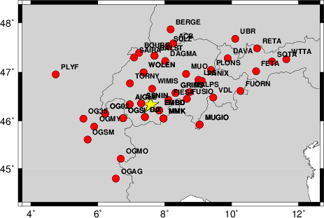
The focal mechanism was determined using broadband seismic waveforms. The location of the event and the and stations used for the waveform inversion are shown in the next figure.
|
|
|
|
The program wvfgrd96 was used with good traces observed at short distance to determine the focal mechanism, depth and seismic moment. This technique requires a high quality signal and well determined velocity model for the Green functions. To the extent that these are the quality data, this type of mechanism should be preferred over the radiation pattern technique which requires the separate step of defining the pressure and tension quadrants and the correct strike.
The observed and predicted traces are filtered using the following gsac commands:
cut o DIST/3.3 -30 o DIST/3.3 +70
rtr
taper w 0.1
hp c 0.02 n 3
lp c 0.06 n 3
The results of this grid search from 0.5 to 19 km depth are as follow:
           DEPTH  STK   DIP  RAKE   MW    FIT
WVFGRD96    1.0   350    85    -5   3.15 0.2804
WVFGRD96    2.0   355    80    10   3.27 0.3696
WVFGRD96    3.0   350    65   -10   3.33 0.3988
WVFGRD96    4.0   350    55   -10   3.38 0.4237
WVFGRD96    5.0   185    45    30   3.46 0.4512
WVFGRD96    6.0   185    45    30   3.49 0.4840
WVFGRD96    7.0   185    50    35   3.51 0.5140
WVFGRD96    8.0   185    45    30   3.55 0.5320
WVFGRD96    9.0   190    45    40   3.58 0.5565
WVFGRD96   10.0   190    45    40   3.60 0.5762
WVFGRD96   11.0   190    45    40   3.62 0.5874
WVFGRD96   12.0   185    50    35   3.61 0.5922
WVFGRD96   13.0   185    50    35   3.62 0.5935
WVFGRD96   14.0   185    55    35   3.62 0.5899
WVFGRD96   15.0   185    55    35   3.63 0.5857
WVFGRD96   16.0   185    55    35   3.64 0.5791
WVFGRD96   17.0   185    55    35   3.64 0.5701
WVFGRD96   18.0   180    60    25   3.63 0.5608
WVFGRD96   19.0   180    60    25   3.64 0.5517
WVFGRD96   20.0   180    60    25   3.65 0.5422
WVFGRD96   21.0   180    60    25   3.65 0.5328
WVFGRD96   22.0   180    60    25   3.66 0.5231
WVFGRD96   23.0   180    60    25   3.66 0.5137
WVFGRD96   24.0   180    60    20   3.67 0.5048
WVFGRD96   25.0   180    65    20   3.67 0.4963
WVFGRD96   26.0   180    65    20   3.67 0.4880
WVFGRD96   27.0   180    65    20   3.68 0.4796
WVFGRD96   28.0   180    65    20   3.68 0.4708
WVFGRD96   29.0   180    65    20   3.69 0.4625
The best solution is
WVFGRD96 13.0 185 50 35 3.62 0.5935
The mechanism correspond to the best fit is
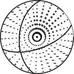
|
|
|
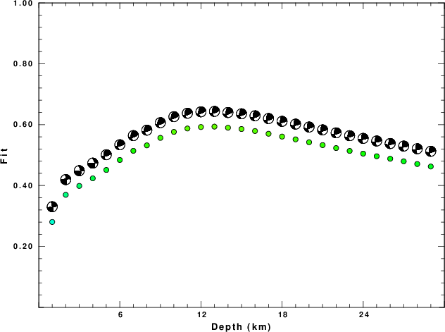
The best fit as a function of depth is given in the following figure:
|
|
|
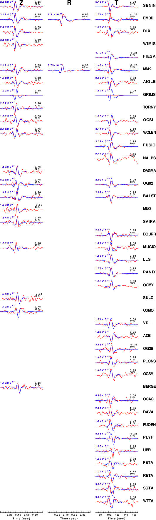
The comparison of the observed and predicted waveforms is given in the next figure. The red traces are the observed and the blue are the predicted. Each observed-predicted component is plotted to the same scale and peak amplitudes are indicated by the numbers to the left of each trace. A pair of numbers is given in black at the right of each predicted traces. The upper number it the time shift required for maximum correlation between the observed and predicted traces. This time shift is required because the synthetics are not computed at exactly the same distance as the observed and because the velocity model used in the predictions may not be perfect. A positive time shift indicates that the prediction is too fast and should be delayed to match the observed trace (shift to the right in this figure). A negative value indicates that the prediction is too slow. The lower number gives the percentage of variance reduction to characterize the individual goodness of fit (100% indicates a perfect fit).
The bandpass filter used in the processing and for the display was
cut o DIST/3.3 -30 o DIST/3.3 +70
rtr
taper w 0.1
hp c 0.02 n 3
lp c 0.06 n 3
|
|
|
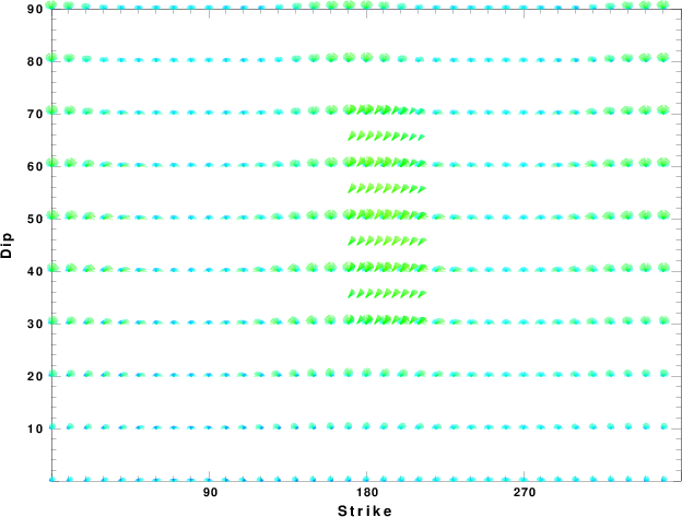
|
| Focal mechanism sensitivity at the preferred depth. The red color indicates a very good fit to thewavefroms. Each solution is plotted as a vector at a given value of strike and dip with the angle of the vector representing the rake angle, measured, with respect to the upward vertical (N) in the figure. |
A check on the assumed source location is possible by looking at the time shifts between the observed and predicted traces. The time shifts for waveform matching arise for several reasons:
Time_shift = A + B cos Azimuth + C Sin Azimuth
The time shifts for this inversion lead to the next figure:
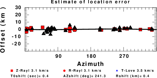
The derived shift in origin time and epicentral coordinates are given at the bottom of the figure.
Should the national backbone of the USGS Advanced National Seismic System (ANSS) be implemented with an interstation separation of 300 km, it is very likely that an earthquake such as this would have been recorded at distances on the order of 100-200 km. This means that the closest station would have information on source depth and mechanism that was lacking here.
Dr. Harley Benz, USGS, provided the USGS USNSN digital data. The digital data used in this study were provided by Natural Resources Canada through their AUTODRM site http://www.seismo.nrcan.gc.ca/nwfa/autodrm/autodrm_req_e.php, and IRIS using their BUD interface.
Thanks also to the many seismic network operators whose dedication make this effort possible: University of Alaska, University of Washington, Oregon State University, University of Utah, Montana Bureas of Mines, UC Berkely, Caltech, UC San Diego, Saint L ouis University, Universityof Memphis, Lamont Doehrty Earth Observatory, Boston College, the Iris stations and the Transportable Array of EarthScope.
The WUS used for the waveform synthetic seismograms and for the surface wave eigenfunctions and dispersion is as follows:
MODEL.01
Model after     8 iterations
ISOTROPIC
KGS
FLAT EARTH
1-D
CONSTANT VELOCITY
LINE08
LINE09
LINE10
LINE11
      H(KM)   VP(KM/S)   VS(KM/S) RHO(GM/CC)         QP         QS       ETAP       ETAS      FREFP      FREFS
     1.9000     3.4065     2.0089     2.2150  0.302E-02  0.679E-02   0.00       0.00       1.00       1.00
     6.1000     5.5445     3.2953     2.6089  0.349E-02  0.784E-02   0.00       0.00       1.00       1.00
    13.0000     6.2708     3.7396     2.7812  0.212E-02  0.476E-02   0.00       0.00       1.00       1.00
    19.0000     6.4075     3.7680     2.8223  0.111E-02  0.249E-02   0.00       0.00       1.00       1.00
     0.0000     7.9000     4.6200     3.2760  0.164E-10  0.370E-10   0.00       0.00       1.00       1.00
Here we tabulate the reasons for not using certain digital data sets
The following stations did not have a valid response files:
DATE=Mon Oct 24 18:01:13 CDT 2016