Location
2016/05/22 08:58:32 41.61 23.30 10 4.5 Bulgaria
Arrival Times (from USGS)
Arrival time list
Felt Map
USGS Felt map for this earthquake
USGS Felt reports archive
Focal Mechanism
 USGS/SLU Moment Tensor Solution
 ENS  2016/05/22 08:58:32:0  41.61   23.30  10.0 4.5 Bulgaria

 Stations used:
   AC.KBN AC.VLO HT.FNA HT.GRG HT.HORT HT.KNT HT.LKD2 HT.SOH
   HT.SRS HT.THE HU.MORH IV.SCTE MN.BLY MN.DIVS MN.TIR MN.VTS
   SJ.BBLS SJ.FRGS

 Filtering commands used:
   cut o DIST/3.3 -30 o DIST/3.3 +70
   rtr
   taper w 0.1
   hp c 0.02 n 3
   lp c 0.06 n 3

 Best Fitting Double Couple
  Mo = 3.80e+22 dyne-cm
  Mw = 4.32
  Z  = 17 km
  Plane   Strike  Dip  Rake
   NP1       38    69   -148
   NP2      295    60   -25
  Principal Axes:
   Axis    Value   Plunge  Azimuth
    T   3.80e+22      5     165
    N   0.00e+00     52      68
    P  -3.80e+22     38     259

 Moment Tensor: (dyne-cm)
    Component   Value
       Mxx     3.43e+22
       Mxy    -1.39e+22
       Mxz     3.97e+15
       Myy    -2.04e+22
       Myz     1.90e+22
       Mzz    -1.39e+22


                     ##############
                 ######################
              ###########################-
             ############################--
           #############################-----
          #####----#####################------
         -------------------###########--------
        ------------------------######----------
        ---------------------------##-----------
       -----------------------------##-----------
       ----------------------------#####---------
       -------   -----------------########-------
       ------- P ----------------###########-----
        ------   --------------##############---
        ----------------------################--
         -------------------###################
          ----------------####################
           -------------#####################
             --------######################
              ---#########################
                 ##############   #####
                     ########## T #


 Global CMT Convention Moment Tensor:
      R          T          P
 -1.39e+22   3.97e+15  -1.90e+22
  3.97e+15   3.43e+22   1.39e+22
 -1.90e+22   1.39e+22  -2.04e+22


Details of the solution is found at

http://www.eas.slu.edu/eqc/eqc_mt/MECH.EU/20160522085832/index.html
|
Preferred Solution
The preferred solution from an analysis of the surface-wave spectral amplitude radiation pattern, waveform inversion and first motion observations is
      STK = 295
      DIP = 60
     RAKE = -25
       MW = 4.32
       HS = 17.0
The NDK file is 20160522085832.ndk
The waveform inversion is preferred.
Moment Tensor Comparison
The following compares this source inversion to others
| SLU |
USGSMT |
 USGS/SLU Moment Tensor Solution
 ENS  2016/05/22 08:58:32:0  41.61   23.30  10.0 4.5 Bulgaria

 Stations used:
   AC.KBN AC.VLO HT.FNA HT.GRG HT.HORT HT.KNT HT.LKD2 HT.SOH
   HT.SRS HT.THE HU.MORH IV.SCTE MN.BLY MN.DIVS MN.TIR MN.VTS
   SJ.BBLS SJ.FRGS

 Filtering commands used:
   cut o DIST/3.3 -30 o DIST/3.3 +70
   rtr
   taper w 0.1
   hp c 0.02 n 3
   lp c 0.06 n 3

 Best Fitting Double Couple
  Mo = 3.80e+22 dyne-cm
  Mw = 4.32
  Z  = 17 km
  Plane   Strike  Dip  Rake
   NP1       38    69   -148
   NP2      295    60   -25
  Principal Axes:
   Axis    Value   Plunge  Azimuth
    T   3.80e+22      5     165
    N   0.00e+00     52      68
    P  -3.80e+22     38     259

 Moment Tensor: (dyne-cm)
    Component   Value
       Mxx     3.43e+22
       Mxy    -1.39e+22
       Mxz     3.97e+15
       Myy    -2.04e+22
       Myz     1.90e+22
       Mzz    -1.39e+22


                     ##############
                 ######################
              ###########################-
             ############################--
           #############################-----
          #####----#####################------
         -------------------###########--------
        ------------------------######----------
        ---------------------------##-----------
       -----------------------------##-----------
       ----------------------------#####---------
       -------   -----------------########-------
       ------- P ----------------###########-----
        ------   --------------##############---
        ----------------------################--
         -------------------###################
          ----------------####################
           -------------#####################
             --------######################
              ---#########################
                 ##############   #####
                     ########## T #


 Global CMT Convention Moment Tensor:
      R          T          P
 -1.39e+22   3.97e+15  -1.90e+22
  3.97e+15   3.43e+22   1.39e+22
 -1.90e+22   1.39e+22  -2.04e+22


Details of the solution is found at

http://www.eas.slu.edu/eqc/eqc_mt/MECH.EU/20160522085832/index.html
|
Regional Moment Tensor (Mwr)
Moment 3.795e+15 N-m
Magnitude 4.3 Mwr
Depth 18.0 km
Percent DC 94 %
Half Duration –
Catalog US
Data Source US1
Contributor US1
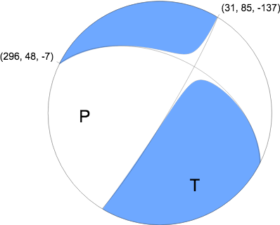
Nodal Planes
Plane Strike Dip Rake
NP1 296 48 -7
NP2 31 85 -137
Principal Axes
Axis Value Plunge Azimuth
T 3.854e+15 N-m 25 156
N -0.121e+15 N-m 47 37
P -3.733e+15 N-m 33 263
|
Waveform Inversion
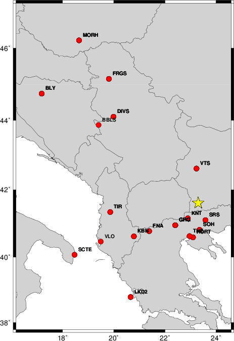
The focal mechanism was determined using broadband seismic waveforms. The location of the event and the
and stations used for the waveform inversion are shown in the next figure.
|
|
Location of broadband stations used for waveform inversion
|
The program wvfgrd96 was used with good traces observed at short distance to determine the focal mechanism, depth and seismic moment. This technique requires a high quality signal and well determined velocity model for the Green functions. To the extent that these are the quality data, this type of mechanism should be preferred over the radiation pattern technique which requires the separate step of defining the pressure and tension quadrants and the correct strike.
The observed and predicted traces are filtered using the following gsac commands:
cut o DIST/3.3 -30 o DIST/3.3 +70
rtr
taper w 0.1
hp c 0.02 n 3
lp c 0.06 n 3
The results of this grid search from 0.5 to 19 km depth are as follow:
           DEPTH  STK   DIP  RAKE   MW    FIT
WVFGRD96    1.0   300    90     5   3.84 0.2786
WVFGRD96    2.0   120    90    -5   3.95 0.3687
WVFGRD96    3.0   300    90     5   4.00 0.4005
WVFGRD96    4.0   130    55    25   4.10 0.4353
WVFGRD96    5.0   130    65    30   4.11 0.4673
WVFGRD96    6.0   125    80    30   4.12 0.5007
WVFGRD96    7.0   300    90   -30   4.14 0.5298
WVFGRD96    8.0   300    85   -35   4.19 0.5638
WVFGRD96    9.0   300    85   -30   4.20 0.5938
WVFGRD96   10.0   290    55   -35   4.26 0.6328
WVFGRD96   11.0   295    60   -30   4.26 0.6700
WVFGRD96   12.0   295    60   -30   4.28 0.6978
WVFGRD96   13.0   295    60   -30   4.29 0.7171
WVFGRD96   14.0   295    60   -30   4.29 0.7298
WVFGRD96   15.0   295    60   -25   4.31 0.7380
WVFGRD96   16.0   295    60   -25   4.31 0.7430
WVFGRD96   17.0   295    60   -25   4.32 0.7444
WVFGRD96   18.0   295    60   -25   4.33 0.7430
WVFGRD96   19.0   300    70   -20   4.32 0.7396
WVFGRD96   20.0   300    70   -20   4.33 0.7356
WVFGRD96   21.0   300    70   -20   4.34 0.7304
WVFGRD96   22.0   300    70   -20   4.34 0.7242
WVFGRD96   23.0   300    70   -20   4.35 0.7165
WVFGRD96   24.0   300    70   -20   4.35 0.7073
WVFGRD96   25.0   300    70   -20   4.36 0.6971
WVFGRD96   26.0   300    70   -20   4.36 0.6873
WVFGRD96   27.0   300    70   -20   4.37 0.6772
WVFGRD96   28.0   300    70   -15   4.38 0.6666
WVFGRD96   29.0   300    70   -15   4.39 0.6555
The best solution is
WVFGRD96 17.0 295 60 -25 4.32 0.7444
The mechanism correspond to the best fit is
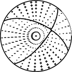
|
|
Figure 1. Waveform inversion focal mechanism
|
The best fit as a function of depth is given in the following figure:
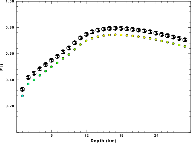
|
|
Figure 2. Depth sensitivity for waveform mechanism
|
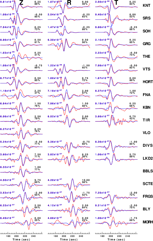
The comparison of the observed and predicted waveforms is given in the next figure. The red traces are the observed and the blue are the predicted.
Each observed-predicted component is plotted to the same scale and peak amplitudes are indicated by the numbers to the left of each trace. A pair of numbers is given in black at the right of each predicted traces. The upper number it the time shift required for maximum correlation between the observed and predicted traces. This time shift is required because the synthetics are not computed at exactly the same distance as the observed and because the velocity model used in the predictions may not be perfect.
A positive time shift indicates that the prediction is too fast and should be delayed to match the observed trace (shift to the right in this figure). A negative value indicates that the prediction is too slow. The lower number gives the percentage of variance reduction to characterize the individual goodness of fit (100% indicates a perfect fit).
The bandpass filter used in the processing and for the display was
cut o DIST/3.3 -30 o DIST/3.3 +70
rtr
taper w 0.1
hp c 0.02 n 3
lp c 0.06 n 3
|
|
Figure 3. Waveform comparison for selected depth
|
|
|
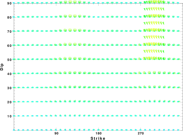
Focal mechanism sensitivity at the preferred depth. The red color indicates a very good fit to thewavefroms.
Each solution is plotted as a vector at a given value of strike and dip with the angle of the vector representing the rake angle, measured, with respect to the upward vertical (N) in the figure.
|
A check on the assumed source location is possible by looking at the time shifts between the observed and predicted traces. The time shifts for waveform matching arise for several reasons:
- The origin time and epicentral distance are incorrect
- The velocity model used for the inversion is incorrect
- The velocity model used to define the P-arrival time is not the
same as the velocity model used for the waveform inversion
(assuming that the initial trace alignment is based on the
P arrival time)
Assuming only a mislocation, the time shifts are fit to a functional form:
Time_shift = A + B cos Azimuth + C Sin Azimuth
The time shifts for this inversion lead to the next figure:
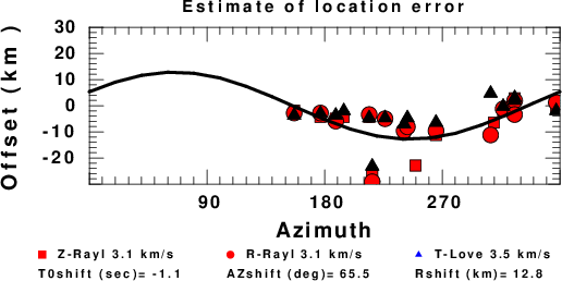
The derived shift in origin time and epicentral coordinates are given at the bottom of the figure.
Discussion
The Future
Should the national backbone of the
USGS Advanced National Seismic System (ANSS)
be implemented with an interstation separation of 300 km, it is very likely that
an earthquake such as this would have been recorded at distances on the order of
100-200 km. This means that the closest station would have information on
source depth and mechanism that was lacking here.
Acknowledgements
Dr. Harley Benz, USGS, provided the USGS USNSN digital data.
The digital data used in this study were provided by Natural Resources Canada through their AUTODRM site http://www.seismo.nrcan.gc.ca/nwfa/autodrm/autodrm_req_e.php, and IRIS using their BUD interface.
Thanks also to the many seismic network operators whose dedication make this effort possible: University of Alaska, University of Washington, Oregon State University, University of Utah, Montana Bureas of Mines, UC Berkely, Caltech, UC San Diego, Saint L ouis University, Universityof Memphis, Lamont Doehrty Earth Observatory, Boston College, the Iris stations and the Transportable Array of EarthScope.
Velocity Model
The WUS used for the waveform synthetic seismograms and for the surface wave eigenfunctions and dispersion is as follows:
MODEL.01
Model after     8 iterations
ISOTROPIC
KGS
FLAT EARTH
1-D
CONSTANT VELOCITY
LINE08
LINE09
LINE10
LINE11
      H(KM)   VP(KM/S)   VS(KM/S) RHO(GM/CC)         QP         QS       ETAP       ETAS      FREFP      FREFS
     1.9000     3.4065     2.0089     2.2150  0.302E-02  0.679E-02   0.00       0.00       1.00       1.00
     6.1000     5.5445     3.2953     2.6089  0.349E-02  0.784E-02   0.00       0.00       1.00       1.00
    13.0000     6.2708     3.7396     2.7812  0.212E-02  0.476E-02   0.00       0.00       1.00       1.00
    19.0000     6.4075     3.7680     2.8223  0.111E-02  0.249E-02   0.00       0.00       1.00       1.00
     0.0000     7.9000     4.6200     3.2760  0.164E-10  0.370E-10   0.00       0.00       1.00       1.00
Quality Control
Here we tabulate the reasons for not using certain digital data sets
The following stations did not have a valid response files:
DATE=Sun May 22 10:26:59 CDT 2016
Last Changed 2016/05/22