2016/04/28 06:46:50 46.06 -1.11 10 5.0 France
USGS Felt map for this earthquake
 USGS/SLU Moment Tensor Solution
 ENS  2016/04/28 06:46:50:0  46.06   -1.11  10.0 5.0 France

 Stations used:
   CH.AIGLE CH.BALST CH.BOURR CH.BRANT CH.DIX CH.EMBD CH.LAUCH
   CH.LKBD2 CH.SAIRA CH.SENIN CH.TORNY CH.VANNI CH.WIMIS
   CH.WOLEN FR.ARBF FR.ATE FR.BANN FR.CALF FR.CAMF FR.CFF
   FR.CHMF FR.FILF FR.FNEB FR.GRN FR.ISO FR.LRVF FR.MLS
   FR.MONQ FR.MVIF FR.OG02 FR.OG35 FR.OGCB FR.OGDI FR.OGMO
   FR.OGMY FR.OGS2 FR.OGS3 FR.OGSA FR.OGSM FR.PAND FR.PYLO
   FR.RENF FR.RSL FR.RUSF FR.SAUF FR.SURF FR.TERF FR.URDF
   FR.VIEF FR.WLS GB.CCA1 GB.DYA GB.ELSH GB.HMNX GB.HTL GB.JSA
   IV.MRGE LC.CANF MN.BNI RD.LOR RD.MTLF RD.ORIF RD.ROSF

 Filtering commands used:
   cut o DIST/3.3 -30 o DIST/3.3 +70
   rtr
   taper w 0.1
   hp c 0.025 n 3
   lp c 0.06 n 3

 Best Fitting Double Couple
  Mo = 9.23e+21 dyne-cm
  Mw = 3.91
  Z  = 14 km
  Plane   Strike  Dip  Rake
   NP1      281    85   -165
   NP2      190    75    -5
  Principal Axes:
   Axis    Value   Plunge  Azimuth
    T   9.23e+21      7      55
    N   0.00e+00     74     299
    P  -9.23e+21     14     147

 Moment Tensor: (dyne-cm)
    Component   Value
       Mxx    -3.02e+21
       Mxy     8.27e+21
       Mxz     2.46e+21
       Myy     3.43e+21
       Myz    -2.73e+20
       Mzz    -4.02e+20


                     ----------####
                 -------------#########
              ---------------#############
             ---------------##############
           ----------------############### T
          -----------------###############   #
         -----------------#####################
        -----------------#######################
        -----------------#######################
       #############-----########################
       #################------###################
       #################--------------###########
       #################---------------------####
        ###############-------------------------
        ###############-------------------------
         ##############------------------------
          #############-----------------------
           ############----------------------
             ##########-------------   ----
              #########------------- P ---
                 #######------------
                     ###-----------


 Global CMT Convention Moment Tensor:
      R          T          P
 -4.02e+20   2.46e+21   2.73e+20
  2.46e+21  -3.02e+21  -8.27e+21
  2.73e+20  -8.27e+21   3.43e+21


Details of the solution is found at

http://www.eas.slu.edu/eqc/eqc_mt/MECH.EU/20160428064650/index.html
|
      STK = 190
      DIP = 75
     RAKE = -5
       MW = 3.91
       HS = 14.0
The NDK file is 20160428064650.ndk The waveform inversion is preferred.
The following compares this source inversion to others
 USGS/SLU Moment Tensor Solution
 ENS  2016/04/28 06:46:50:0  46.06   -1.11  10.0 5.0 France

 Stations used:
   CH.AIGLE CH.BALST CH.BOURR CH.BRANT CH.DIX CH.EMBD CH.LAUCH
   CH.LKBD2 CH.SAIRA CH.SENIN CH.TORNY CH.VANNI CH.WIMIS
   CH.WOLEN FR.ARBF FR.ATE FR.BANN FR.CALF FR.CAMF FR.CFF
   FR.CHMF FR.FILF FR.FNEB FR.GRN FR.ISO FR.LRVF FR.MLS
   FR.MONQ FR.MVIF FR.OG02 FR.OG35 FR.OGCB FR.OGDI FR.OGMO
   FR.OGMY FR.OGS2 FR.OGS3 FR.OGSA FR.OGSM FR.PAND FR.PYLO
   FR.RENF FR.RSL FR.RUSF FR.SAUF FR.SURF FR.TERF FR.URDF
   FR.VIEF FR.WLS GB.CCA1 GB.DYA GB.ELSH GB.HMNX GB.HTL GB.JSA
   IV.MRGE LC.CANF MN.BNI RD.LOR RD.MTLF RD.ORIF RD.ROSF

 Filtering commands used:
   cut o DIST/3.3 -30 o DIST/3.3 +70
   rtr
   taper w 0.1
   hp c 0.025 n 3
   lp c 0.06 n 3

 Best Fitting Double Couple
  Mo = 9.23e+21 dyne-cm
  Mw = 3.91
  Z  = 14 km
  Plane   Strike  Dip  Rake
   NP1      281    85   -165
   NP2      190    75    -5
  Principal Axes:
   Axis    Value   Plunge  Azimuth
    T   9.23e+21      7      55
    N   0.00e+00     74     299
    P  -9.23e+21     14     147

 Moment Tensor: (dyne-cm)
    Component   Value
       Mxx    -3.02e+21
       Mxy     8.27e+21
       Mxz     2.46e+21
       Myy     3.43e+21
       Myz    -2.73e+20
       Mzz    -4.02e+20


                     ----------####
                 -------------#########
              ---------------#############
             ---------------##############
           ----------------############### T
          -----------------###############   #
         -----------------#####################
        -----------------#######################
        -----------------#######################
       #############-----########################
       #################------###################
       #################--------------###########
       #################---------------------####
        ###############-------------------------
        ###############-------------------------
         ##############------------------------
          #############-----------------------
           ############----------------------
             ##########-------------   ----
              #########------------- P ---
                 #######------------
                     ###-----------


 Global CMT Convention Moment Tensor:
      R          T          P
 -4.02e+20   2.46e+21   2.73e+20
  2.46e+21  -3.02e+21  -8.27e+21
  2.73e+20  -8.27e+21   3.43e+21


Details of the solution is found at

http://www.eas.slu.edu/eqc/eqc_mt/MECH.EU/20160428064650/index.html
|
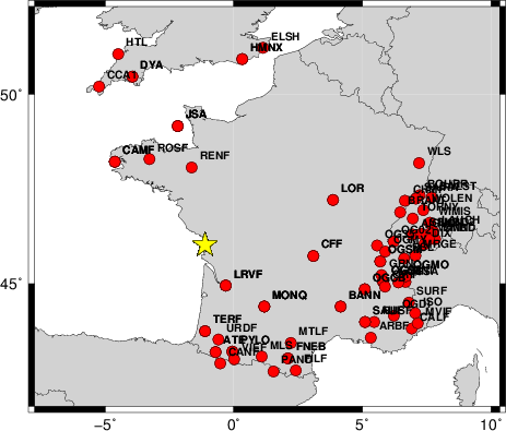
The focal mechanism was determined using broadband seismic waveforms. The location of the event and the and stations used for the waveform inversion are shown in the next figure.
|
|
|
|
The program wvfgrd96 was used with good traces observed at short distance to determine the focal mechanism, depth and seismic moment. This technique requires a high quality signal and well determined velocity model for the Green functions. To the extent that these are the quality data, this type of mechanism should be preferred over the radiation pattern technique which requires the separate step of defining the pressure and tension quadrants and the correct strike.
The observed and predicted traces are filtered using the following gsac commands:
cut o DIST/3.3 -30 o DIST/3.3 +70
rtr
taper w 0.1
hp c 0.025 n 3
lp c 0.06 n 3
The results of this grid search from 0.5 to 19 km depth are as follow:
           DEPTH  STK   DIP  RAKE   MW    FIT
WVFGRD96    1.0     0    60   -30   3.68 0.3360
WVFGRD96    2.0   180    60   -30   3.74 0.3862
WVFGRD96    3.0   180    60   -35   3.78 0.4131
WVFGRD96    4.0   180    60   -35   3.80 0.4344
WVFGRD96    5.0   180    60   -30   3.80 0.4504
WVFGRD96    6.0   185    65   -15   3.79 0.4656
WVFGRD96    7.0   185    70   -15   3.80 0.4813
WVFGRD96    8.0   185    65   -15   3.84 0.4986
WVFGRD96    9.0   185    65   -15   3.85 0.5102
WVFGRD96   10.0   185    70   -15   3.86 0.5191
WVFGRD96   11.0   185    70   -10   3.87 0.5259
WVFGRD96   12.0   190    70    -5   3.89 0.5309
WVFGRD96   13.0   190    75    -5   3.90 0.5339
WVFGRD96   14.0   190    75    -5   3.91 0.5347
WVFGRD96   15.0   190    75    -5   3.92 0.5328
WVFGRD96   16.0   190    80   -10   3.93 0.5295
WVFGRD96   17.0   190    80   -10   3.94 0.5245
WVFGRD96   18.0   190    80   -10   3.94 0.5180
WVFGRD96   19.0   190    80   -10   3.95 0.5103
WVFGRD96   20.0   190    80   -10   3.96 0.5016
WVFGRD96   21.0   185    75   -10   3.95 0.4925
WVFGRD96   22.0   185    75   -10   3.96 0.4826
WVFGRD96   23.0   185    75   -10   3.97 0.4723
WVFGRD96   24.0   185    80   -15   3.97 0.4615
WVFGRD96   25.0   185    80   -15   3.98 0.4506
WVFGRD96   26.0   185    80   -15   3.98 0.4395
WVFGRD96   27.0   185    80   -15   3.99 0.4282
WVFGRD96   28.0    10    90     5   4.00 0.4157
WVFGRD96   29.0   100    90    -5   4.01 0.4087
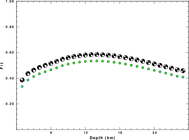
The best solution is
WVFGRD96 14.0 190 75 -5 3.91 0.5347
The mechanism correspond to the best fit is
|
|
|
The best fit as a function of depth is given in the following figure:
|
|
|
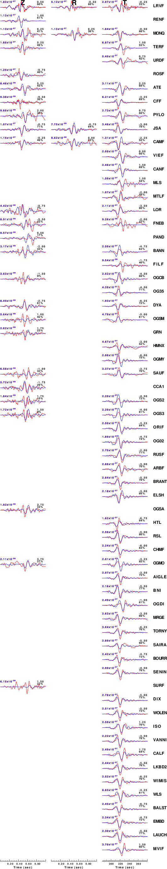
The comparison of the observed and predicted waveforms is given in the next figure. The red traces are the observed and the blue are the predicted. Each observed-predicted component is plotted to the same scale and peak amplitudes are indicated by the numbers to the left of each trace. A pair of numbers is given in black at the right of each predicted traces. The upper number it the time shift required for maximum correlation between the observed and predicted traces. This time shift is required because the synthetics are not computed at exactly the same distance as the observed and because the velocity model used in the predictions may not be perfect. A positive time shift indicates that the prediction is too fast and should be delayed to match the observed trace (shift to the right in this figure). A negative value indicates that the prediction is too slow. The lower number gives the percentage of variance reduction to characterize the individual goodness of fit (100% indicates a perfect fit).
The bandpass filter used in the processing and for the display was
cut o DIST/3.3 -30 o DIST/3.3 +70
rtr
taper w 0.1
hp c 0.025 n 3
lp c 0.06 n 3
|
|
|
|
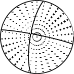
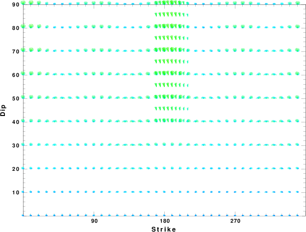
| Focal mechanism sensitivity at the preferred depth. The red color indicates a very good fit to thewavefroms. Each solution is plotted as a vector at a given value of strike and dip with the angle of the vector representing the rake angle, measured, with respect to the upward vertical (N) in the figure. |
A check on the assumed source location is possible by looking at the time shifts between the observed and predicted traces. The time shifts for waveform matching arise for several reasons:
Time_shift = A + B cos Azimuth + C Sin Azimuth
The time shifts for this inversion lead to the next figure:
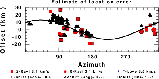
The derived shift in origin time and epicentral coordinates are given at the bottom of the figure.
Should the national backbone of the USGS Advanced National Seismic System (ANSS) be implemented with an interstation separation of 300 km, it is very likely that an earthquake such as this would have been recorded at distances on the order of 100-200 km. This means that the closest station would have information on source depth and mechanism that was lacking here.
Dr. Harley Benz, USGS, provided the USGS USNSN digital data. The digital data used in this study were provided by Natural Resources Canada through their AUTODRM site http://www.seismo.nrcan.gc.ca/nwfa/autodrm/autodrm_req_e.php, and IRIS using their BUD interface.
Thanks also to the many seismic network operators whose dedication make this effort possible: University of Alaska, University of Washington, Oregon State University, University of Utah, Montana Bureas of Mines, UC Berkely, Caltech, UC San Diego, Saint L ouis University, Universityof Memphis, Lamont Doehrty Earth Observatory, Boston College, the Iris stations and the Transportable Array of EarthScope.
The WUS used for the waveform synthetic seismograms and for the surface wave eigenfunctions and dispersion is as follows:
MODEL.01
Model after     8 iterations
ISOTROPIC
KGS
FLAT EARTH
1-D
CONSTANT VELOCITY
LINE08
LINE09
LINE10
LINE11
      H(KM)   VP(KM/S)   VS(KM/S) RHO(GM/CC)         QP         QS       ETAP       ETAS      FREFP      FREFS
     1.9000     3.4065     2.0089     2.2150  0.302E-02  0.679E-02   0.00       0.00       1.00       1.00
     6.1000     5.5445     3.2953     2.6089  0.349E-02  0.784E-02   0.00       0.00       1.00       1.00
    13.0000     6.2708     3.7396     2.7812  0.212E-02  0.476E-02   0.00       0.00       1.00       1.00
    19.0000     6.4075     3.7680     2.8223  0.111E-02  0.249E-02   0.00       0.00       1.00       1.00
     0.0000     7.9000     4.6200     3.2760  0.164E-10  0.370E-10   0.00       0.00       1.00       1.00
Here we tabulate the reasons for not using certain digital data sets
The following stations did not have a valid response files:
DATE=Thu Apr 28 13:53:46 CDT 2016