Location
Location ANSS
2015/02/23 16:16:29 39.04 -2.65 10.0 4.8 Spain
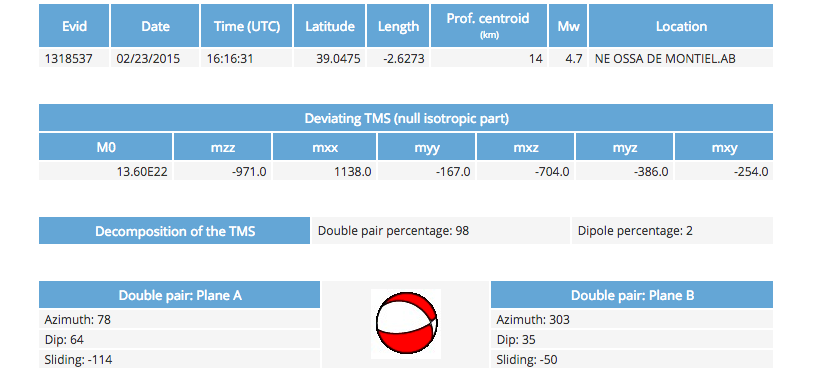
Focal Mechanism
 USGS/SLU Moment Tensor Solution
 ENS  2015/02/23 16:16:29:0  39.04   -2.65  10.0 4.8 Spain

 Stations used:
   CA.CAVN CA.CBEU CA.CMAS CA.CORG CA.CPAL CA.CTRE ES.EADA
   ES.EALB ES.EARI ES.EBER ES.EGRO ES.EIBI ES.ELAN ES.ELGU
   ES.ELOB ES.EMIN ES.EMOS ES.EMUR ES.ENIJ ES.EORO ES.EPLA
   ES.EPOB ES.EQES ES.EQTA ES.ERTA ES.ESAC ES.ESBB SC.SC02
   SC.SC03 SC.SC04 SC.SC05 SC.SC06 SC.SC08 SC.SC09 SC.SC10
   SC.SC11 SC.SC12 SC.SC13 SC.SC14 SC.SC15 SC.SC16 SC.SC17
   SC.SC18 SC.SC20 SC.SC21 SC.SC22 SC.SC23 SC.SC24 SC.SC25
   SC.SC26 SC.SC27 SC.SC28 SC.SC30

 Filtering commands used:
   cut o DIST/3.3 -30 o DIST/3.3 +70
   rtr
   taper w 0.1
   hp c 0.03 n 3
   lp c 0.10 n 3

 Best Fitting Double Couple
  Mo = 9.02e+22 dyne-cm
  Mw = 4.57
  Z  = 18 km
  Plane   Strike  Dip  Rake
   NP1      248    73   -132
   NP2      140    45   -25
  Principal Axes:
   Axis    Value   Plunge  Azimuth
    T   9.02e+22     17       8
    N   0.00e+00     40     263
    P  -9.02e+22     45     116

 Moment Tensor: (dyne-cm)
    Component   Value
       Mxx     7.26e+22
       Mxy     2.88e+22
       Mxz     4.43e+22
       Myy    -3.45e+22
       Myz    -3.71e+22
       Mzz    -3.81e+22


                     ########   ###
                 ############ T #######
              -##############   ##########
             -#############################
           --################################
          ---#################################
         ----##################################
        -----####################---------------
        ------##############--------------------
       -------#########--------------------------
       --------#####-----------------------------
       --------#---------------------------------
       -------##--------------------   ----------
        ----#####------------------- P ---------
        --#########-----------------   ---------
         ###########---------------------------
          ############------------------------
           ##############--------------------
             ###############---------------
              ##################----------
                 ######################
                     ##############


 Global CMT Convention Moment Tensor:
      R          T          P
 -3.81e+22   4.43e+22   3.71e+22
  4.43e+22   7.26e+22  -2.88e+22
  3.71e+22  -2.88e+22  -3.45e+22


Details of the solution is found at

http://www.eas.slu.edu/eqc/eqc_mt/MECH.NA/20150223161629/index.html
|
Preferred Solution
The preferred solution from an analysis of the surface-wave spectral amplitude radiation pattern, waveform inversion and first motion observations is
      STK = 140
      DIP = 45
     RAKE = -25
       MW = 4.57
       HS = 18.0
The NDK file is 20150223161629.ndk
The waveform inversion is preferred.
Moment Tensor Comparison
The following compares this source inversion to others
| SLU |
IGN |
 USGS/SLU Moment Tensor Solution
 ENS  2015/02/23 16:16:29:0  39.04   -2.65  10.0 4.8 Spain

 Stations used:
   CA.CAVN CA.CBEU CA.CMAS CA.CORG CA.CPAL CA.CTRE ES.EADA
   ES.EALB ES.EARI ES.EBER ES.EGRO ES.EIBI ES.ELAN ES.ELGU
   ES.ELOB ES.EMIN ES.EMOS ES.EMUR ES.ENIJ ES.EORO ES.EPLA
   ES.EPOB ES.EQES ES.EQTA ES.ERTA ES.ESAC ES.ESBB SC.SC02
   SC.SC03 SC.SC04 SC.SC05 SC.SC06 SC.SC08 SC.SC09 SC.SC10
   SC.SC11 SC.SC12 SC.SC13 SC.SC14 SC.SC15 SC.SC16 SC.SC17
   SC.SC18 SC.SC20 SC.SC21 SC.SC22 SC.SC23 SC.SC24 SC.SC25
   SC.SC26 SC.SC27 SC.SC28 SC.SC30

 Filtering commands used:
   cut o DIST/3.3 -30 o DIST/3.3 +70
   rtr
   taper w 0.1
   hp c 0.03 n 3
   lp c 0.10 n 3

 Best Fitting Double Couple
  Mo = 9.02e+22 dyne-cm
  Mw = 4.57
  Z  = 18 km
  Plane   Strike  Dip  Rake
   NP1      248    73   -132
   NP2      140    45   -25
  Principal Axes:
   Axis    Value   Plunge  Azimuth
    T   9.02e+22     17       8
    N   0.00e+00     40     263
    P  -9.02e+22     45     116

 Moment Tensor: (dyne-cm)
    Component   Value
       Mxx     7.26e+22
       Mxy     2.88e+22
       Mxz     4.43e+22
       Myy    -3.45e+22
       Myz    -3.71e+22
       Mzz    -3.81e+22


                     ########   ###
                 ############ T #######
              -##############   ##########
             -#############################
           --################################
          ---#################################
         ----##################################
        -----####################---------------
        ------##############--------------------
       -------#########--------------------------
       --------#####-----------------------------
       --------#---------------------------------
       -------##--------------------   ----------
        ----#####------------------- P ---------
        --#########-----------------   ---------
         ###########---------------------------
          ############------------------------
           ##############--------------------
             ###############---------------
              ##################----------
                 ######################
                     ##############


 Global CMT Convention Moment Tensor:
      R          T          P
 -3.81e+22   4.43e+22   3.71e+22
  4.43e+22   7.26e+22  -2.88e+22
  3.71e+22  -2.88e+22  -3.45e+22


Details of the solution is found at

http://www.eas.slu.edu/eqc/eqc_mt/MECH.NA/20150223161629/index.html
|
|
Magnitudes
mLg Magnitude
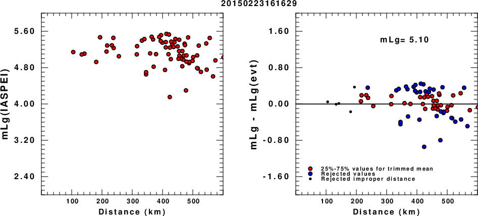
(a) mLg computed using the IASPEI formula; (b) mLg residuals ; the values used for the trimmed mean are indicated.
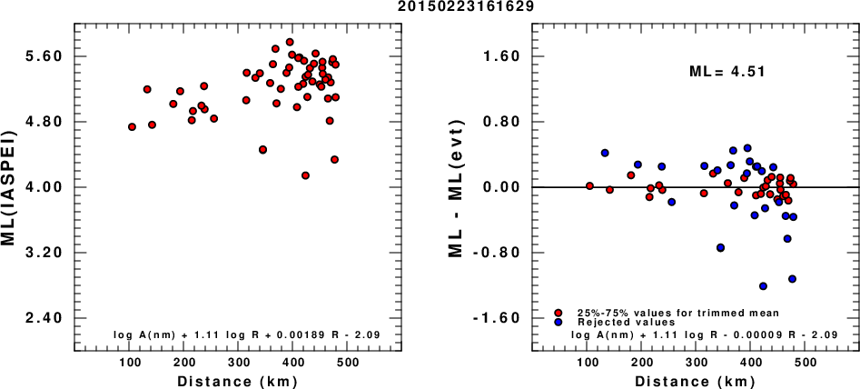
ML Magnitude
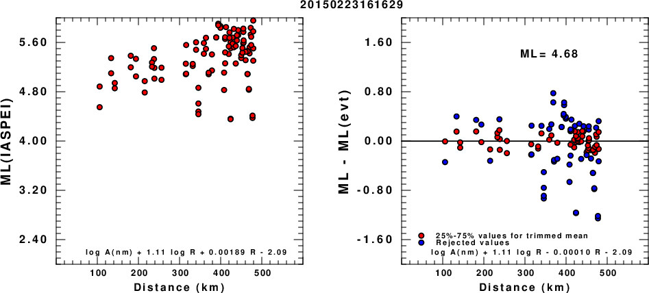
(a) ML computed using the IASPEI formula for Horizontal components; (b) ML residuals computed using a modified IASPEI formula that accounts for path specific attenuation; the values used for the trimmed mean are indicated. The ML relation used for each figure is given at the bottom of each plot.
(a) ML computed using the IASPEI formula for Vertical components (research); (b) ML residuals computed using a modified IASPEI formula that accounts for path specific attenuation; the values used for the trimmed mean are indicated. The ML relation used for each figure is given at the bottom of each plot.
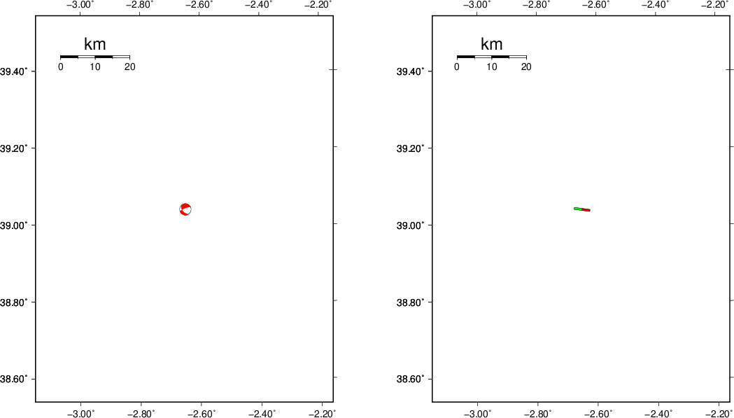
Context
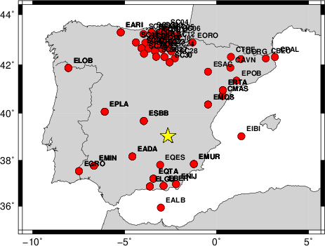
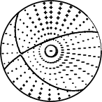
The next figure presents the focal mechanism for this earthquake (red) in the context of other events (blue) in the SLU Moment Tensor Catalog which are within ± 0.5 degrees of the new event. This comparison is shown in the left panel of the figure. The right panel shows the inferred direction of maximum compressive stress and the type of faulting (green is strike-slip, red is normal, blue is thrust; oblique is shown by a combination of colors).
Waveform Inversion using wvfgrd96
The focal mechanism was determined using broadband seismic waveforms. The location of the event and the
and stations used for the waveform inversion are shown in the next figure.
|
|
Location of broadband stations used for waveform inversion
|
The program wvfgrd96 was used with good traces observed at short distance to determine the focal mechanism, depth and seismic moment. This technique requires a high quality signal and well determined velocity model for the Green functions. To the extent that these are the quality data, this type of mechanism should be preferred over the radiation pattern technique which requires the separate step of defining the pressure and tension quadrants and the correct strike.
The observed and predicted traces are filtered using the following gsac commands:
cut o DIST/3.3 -30 o DIST/3.3 +70
rtr
taper w 0.1
hp c 0.03 n 3
lp c 0.10 n 3
The results of this grid search from 0.5 to 19 km depth are as follow:
           DEPTH  STK   DIP  RAKE   MW    FIT
WVFGRD96    1.0    70    45    90   4.15 0.2542
WVFGRD96    2.0   250    45    90   4.27 0.3094
WVFGRD96    3.0    70    80    20   4.23 0.2463
WVFGRD96    4.0   245    80   -45   4.29 0.2466
WVFGRD96    5.0    65    90    55   4.30 0.2777
WVFGRD96    6.0    65    90    55   4.31 0.3097
WVFGRD96    7.0   245    90   -55   4.32 0.3354
WVFGRD96    8.0    65    85    60   4.40 0.3550
WVFGRD96    9.0   250    80    60   4.41 0.3802
WVFGRD96   10.0   250    80    60   4.43 0.4026
WVFGRD96   11.0   250    80    60   4.44 0.4206
WVFGRD96   12.0   250    75    60   4.46 0.4337
WVFGRD96   13.0   245    80    60   4.47 0.4442
WVFGRD96   14.0   245    80    60   4.49 0.4510
WVFGRD96   15.0   135    45   -35   4.53 0.4553
WVFGRD96   16.0   135    45   -35   4.55 0.4627
WVFGRD96   17.0   135    45   -35   4.56 0.4663
WVFGRD96   18.0   140    45   -25   4.57 0.4665
WVFGRD96   19.0   140    45   -25   4.58 0.4646
WVFGRD96   20.0   140    45   -25   4.60 0.4602
WVFGRD96   21.0   140    40   -25   4.60 0.4525
WVFGRD96   22.0   135    40   -25   4.61 0.4447
WVFGRD96   23.0   135    40   -25   4.62 0.4351
WVFGRD96   24.0   135    40   -25   4.63 0.4239
WVFGRD96   25.0   135    35   -20   4.64 0.4113
WVFGRD96   26.0   135    35   -20   4.64 0.3987
WVFGRD96   27.0   140    35   -15   4.65 0.3850
WVFGRD96   28.0   135    30   -20   4.65 0.3710
WVFGRD96   29.0   135    30   -20   4.66 0.3561
The best solution is
WVFGRD96 18.0 140 45 -25 4.57 0.4665
The mechanism correspond to the best fit is
|
|
Figure 1. Waveform inversion focal mechanism
|
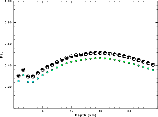
The best fit as a function of depth is given in the following figure:
|
|
Figure 2. Depth sensitivity for waveform mechanism
|
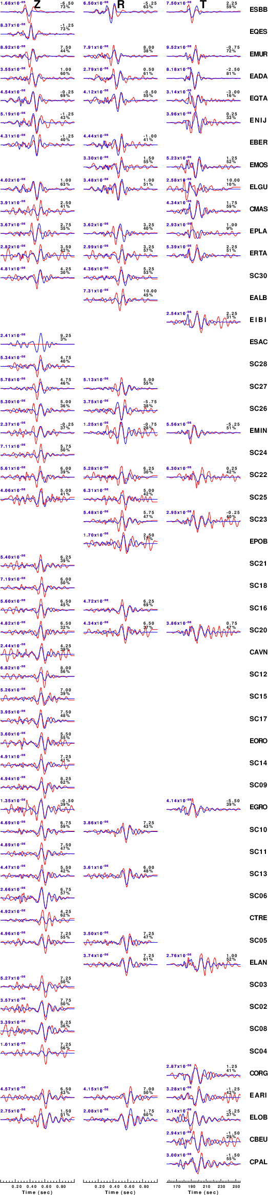
The comparison of the observed and predicted waveforms is given in the next figure. The red traces are the observed and the blue are the predicted.
Each observed-predicted component is plotted to the same scale and peak amplitudes are indicated by the numbers to the left of each trace. A pair of numbers is given in black at the right of each predicted traces. The upper number it the time shift required for maximum correlation between the observed and predicted traces. This time shift is required because the synthetics are not computed at exactly the same distance as the observed and because the velocity model used in the predictions may not be perfect.
A positive time shift indicates that the prediction is too fast and should be delayed to match the observed trace (shift to the right in this figure). A negative value indicates that the prediction is too slow. The lower number gives the percentage of variance reduction to characterize the individual goodness of fit (100% indicates a perfect fit).
The bandpass filter used in the processing and for the display was
cut o DIST/3.3 -30 o DIST/3.3 +70
rtr
taper w 0.1
hp c 0.03 n 3
lp c 0.10 n 3
|
|
Figure 3. Waveform comparison for selected depth. Red: observed; Blue - predicted. The time shift with respect to the model prediction is indicated. The percent of fit is also indicated.
|
|
|
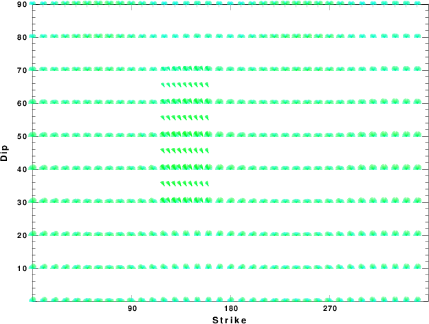
Focal mechanism sensitivity at the preferred depth. The red color indicates a very good fit to thewavefroms.
Each solution is plotted as a vector at a given value of strike and dip with the angle of the vector representing the rake angle, measured, with respect to the upward vertical (N) in the figure.
|
A check on the assumed source location is possible by looking at the time shifts between the observed and predicted traces. The time shifts for waveform matching arise for several reasons:
- The origin time and epicentral distance are incorrect
- The velocity model used for the inversion is incorrect
- The velocity model used to define the P-arrival time is not the
same as the velocity model used for the waveform inversion
(assuming that the initial trace alignment is based on the
P arrival time)
Assuming only a mislocation, the time shifts are fit to a functional form:
Time_shift = A + B cos Azimuth + C Sin Azimuth
The time shifts for this inversion lead to the next figure:
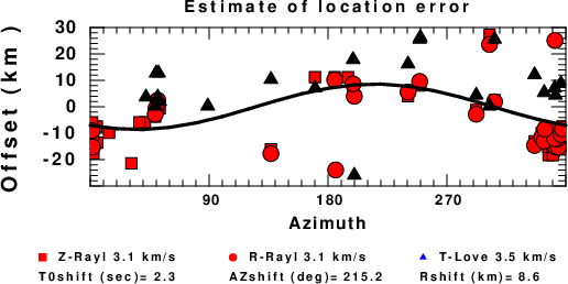
The derived shift in origin time and epicentral coordinates are given at the bottom of the figure.
Discussion
Acknowledgements
Thanks also to the many seismic network operators whose dedication make this effort possible: University of Nevada Reno, University of Alaska, University of Washington, Oregon State University, University of Utah, Montana Bureas of Mines, UC Berkely, Caltech, UC San Diego, Saint Louis University, University of Memphis, Lamont Doherty Earth Observatory, the Iris stations and the Transportable Array of EarthScope.
Velocity Model
The CUS.model used for the waveform synthetic seismograms and for the surface wave eigenfunctions and dispersion is as follows:
MODEL.01
CUS Model with Q from simple gamma values
ISOTROPIC
KGS
FLAT EARTH
1-D
CONSTANT VELOCITY
LINE08
LINE09
LINE10
LINE11
  H(KM) VP(KM/S) VS(KM/S) RHO(GM/CC)   QP   QS  ETAP  ETAS  FREFP  FREFS
  1.0000  5.0000  2.8900  2.5000 0.172E-02 0.387E-02 0.00  0.00  1.00  1.00
  9.0000  6.1000  3.5200  2.7300 0.160E-02 0.363E-02 0.00  0.00  1.00  1.00
 10.0000  6.4000  3.7000  2.8200 0.149E-02 0.336E-02 0.00  0.00  1.00  1.00
 20.0000  6.7000  3.8700  2.9020 0.000E-04 0.000E-04 0.00  0.00  1.00  1.00
  0.0000  8.1500  4.7000  3.3640 0.194E-02 0.431E-02 0.00  0.00  1.00  1.00
Quality Control
Here we tabulate the reasons for not using certain digital data sets
The following stations did not have a valid response files:
Last Changed Sat Jun 23 04:34:13 CDT 2018