2015/02/23 16:16:29 39.04 -2.65 10 4.8 Spain
USGS Felt map for this earthquake
 USGS/SLU Moment Tensor Solution
 ENS  2015/02/23 16:16:29:0  39.04   -2.65  10.0 4.8 Spain

 Stations used:
   FR.ATE FR.FILF FR.MLS FR.SJAF FR.VIEF GE.MTE IU.PAB
   PM.PESTR PM.PFVI PM.PVAQ RD.MTLF SS.COI WM.CART

 Filtering commands used:
   cut o DIST/3.3 -30 o DIST/3.3 +70
   rtr
   taper w 0.1
   hp c 0.02 n 3
   lp c 0.06 n 3

 Best Fitting Double Couple
  Mo = 6.84e+22 dyne-cm
  Mw = 4.49
  Z  = 13 km
  Plane   Strike  Dip  Rake
   NP1       77    63   -121
   NP2      310    40   -45
  Principal Axes:
   Axis    Value   Plunge  Azimuth
    T   6.84e+22     13     189
    N   0.00e+00     27      93
    P  -6.84e+22     60     302

 Moment Tensor: (dyne-cm)
    Component   Value
       Mxx     5.86e+22
       Mxy     1.81e+22
       Mxz    -3.02e+22
       Myy    -1.09e+22
       Myz     2.30e+22
       Mzz    -4.76e+22


                     ##############
                 ######################
              ############################
             ----------------##############
           ---------------------#############
          -------------------------###########
         ----------------------------##########
        -----------   -----------------#########
        ----------- P ------------------########
       ------------   --------------------#####--
       ------------------------------------##----
       ------------------------------------------
       ---------------------------------####-----
        ----------------------------########----
        ####------------------###############---
         ####################################--
          ###################################-
           #################################-
             ##############################
              ##########   ###############
                 ####### T ############
                     ###   ########


 Global CMT Convention Moment Tensor:
      R          T          P
 -4.76e+22  -3.02e+22  -2.30e+22
 -3.02e+22   5.86e+22  -1.81e+22
 -2.30e+22  -1.81e+22  -1.09e+22


Details of the solution is found at

http://www.eas.slu.edu/eqc/eqc_mt/MECH.EU/20150223161629/index.html
|
      STK = 310
      DIP = 40
     RAKE = -45
       MW = 4.49
       HS = 13.0
The NDK file is 20150223161629.ndk The waveform inversion is preferred.
The following compares this source inversion to others
 USGS/SLU Moment Tensor Solution
 ENS  2015/02/23 16:16:29:0  39.04   -2.65  10.0 4.8 Spain

 Stations used:
   FR.ATE FR.FILF FR.MLS FR.SJAF FR.VIEF GE.MTE IU.PAB
   PM.PESTR PM.PFVI PM.PVAQ RD.MTLF SS.COI WM.CART

 Filtering commands used:
   cut o DIST/3.3 -30 o DIST/3.3 +70
   rtr
   taper w 0.1
   hp c 0.02 n 3
   lp c 0.06 n 3

 Best Fitting Double Couple
  Mo = 6.84e+22 dyne-cm
  Mw = 4.49
  Z  = 13 km
  Plane   Strike  Dip  Rake
   NP1       77    63   -121
   NP2      310    40   -45
  Principal Axes:
   Axis    Value   Plunge  Azimuth
    T   6.84e+22     13     189
    N   0.00e+00     27      93
    P  -6.84e+22     60     302

 Moment Tensor: (dyne-cm)
    Component   Value
       Mxx     5.86e+22
       Mxy     1.81e+22
       Mxz    -3.02e+22
       Myy    -1.09e+22
       Myz     2.30e+22
       Mzz    -4.76e+22


                     ##############
                 ######################
              ############################
             ----------------##############
           ---------------------#############
          -------------------------###########
         ----------------------------##########
        -----------   -----------------#########
        ----------- P ------------------########
       ------------   --------------------#####--
       ------------------------------------##----
       ------------------------------------------
       ---------------------------------####-----
        ----------------------------########----
        ####------------------###############---
         ####################################--
          ###################################-
           #################################-
             ##############################
              ##########   ###############
                 ####### T ############
                     ###   ########


 Global CMT Convention Moment Tensor:
      R          T          P
 -4.76e+22  -3.02e+22  -2.30e+22
 -3.02e+22   5.86e+22  -1.81e+22
 -2.30e+22  -1.81e+22  -1.09e+22


Details of the solution is found at

http://www.eas.slu.edu/eqc/eqc_mt/MECH.EU/20150223161629/index.html
|
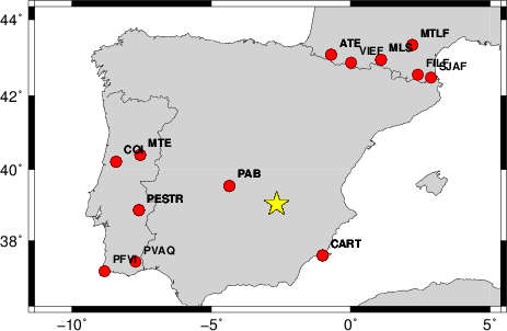
The focal mechanism was determined using broadband seismic waveforms. The location of the event and the and stations used for the waveform inversion are shown in the next figure.
|
|
|
|
The program wvfgrd96 was used with good traces observed at short distance to determine the focal mechanism, depth and seismic moment. This technique requires a high quality signal and well determined velocity model for the Green functions. To the extent that these are the quality data, this type of mechanism should be preferred over the radiation pattern technique which requires the separate step of defining the pressure and tension quadrants and the correct strike.
The observed and predicted traces are filtered using the following gsac commands:
cut o DIST/3.3 -30 o DIST/3.3 +70
rtr
taper w 0.1
hp c 0.02 n 3
lp c 0.06 n 3
The results of this grid search from 0.5 to 19 km depth are as follow:
           DEPTH  STK   DIP  RAKE   MW    FIT
WVFGRD96    1.0   340    85    -5   4.15 0.4183
WVFGRD96    2.0   160    90     5   4.23 0.4684
WVFGRD96    3.0   160    85     5   4.28 0.4798
WVFGRD96    4.0   320    45   -25   4.36 0.4962
WVFGRD96    5.0   320    45   -25   4.37 0.5443
WVFGRD96    6.0   320    45   -25   4.38 0.5830
WVFGRD96    7.0   320    45   -25   4.38 0.6107
WVFGRD96    8.0   320    40   -25   4.44 0.6352
WVFGRD96    9.0   320    40   -25   4.45 0.6604
WVFGRD96   10.0   315    40   -35   4.47 0.6818
WVFGRD96   11.0   310    40   -45   4.49 0.6964
WVFGRD96   12.0   310    40   -45   4.49 0.7058
WVFGRD96   13.0   310    40   -45   4.49 0.7091
WVFGRD96   14.0   315    45   -35   4.48 0.7090
WVFGRD96   15.0   315    45   -35   4.49 0.7062
WVFGRD96   16.0   315    45   -35   4.50 0.7010
WVFGRD96   17.0   320    50   -25   4.50 0.6943
WVFGRD96   18.0   320    50   -25   4.50 0.6859
WVFGRD96   19.0   320    50   -25   4.51 0.6759
WVFGRD96   20.0   320    55   -30   4.53 0.6657
WVFGRD96   21.0   320    55   -30   4.54 0.6560
WVFGRD96   22.0   320    55   -30   4.55 0.6441
WVFGRD96   23.0   320    55   -30   4.55 0.6314
WVFGRD96   24.0   320    55   -30   4.56 0.6181
WVFGRD96   25.0   320    60   -30   4.57 0.6047
WVFGRD96   26.0   320    60   -30   4.57 0.5915
WVFGRD96   27.0   320    60   -30   4.58 0.5777
WVFGRD96   28.0   320    60   -30   4.59 0.5637
WVFGRD96   29.0   320    60   -30   4.59 0.5493
The best solution is
WVFGRD96 13.0 310 40 -45 4.49 0.7091
The mechanism correspond to the best fit is
|
|
|
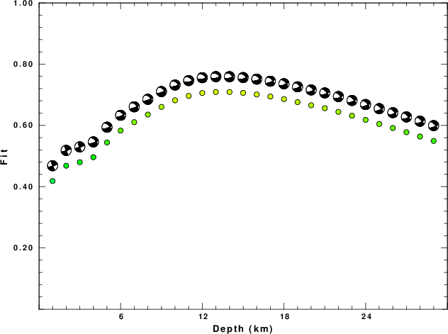
The best fit as a function of depth is given in the following figure:
|
|
|
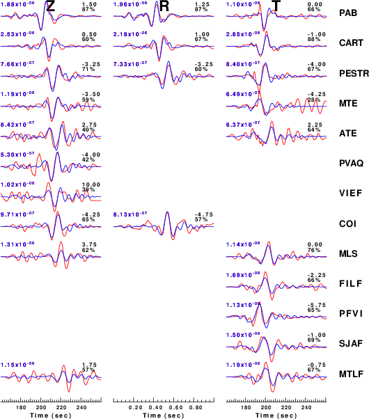
The comparison of the observed and predicted waveforms is given in the next figure. The red traces are the observed and the blue are the predicted. Each observed-predicted component is plotted to the same scale and peak amplitudes are indicated by the numbers to the left of each trace. A pair of numbers is given in black at the right of each predicted traces. The upper number it the time shift required for maximum correlation between the observed and predicted traces. This time shift is required because the synthetics are not computed at exactly the same distance as the observed and because the velocity model used in the predictions may not be perfect. A positive time shift indicates that the prediction is too fast and should be delayed to match the observed trace (shift to the right in this figure). A negative value indicates that the prediction is too slow. The lower number gives the percentage of variance reduction to characterize the individual goodness of fit (100% indicates a perfect fit).
The bandpass filter used in the processing and for the display was
cut o DIST/3.3 -30 o DIST/3.3 +70
rtr
taper w 0.1
hp c 0.02 n 3
lp c 0.06 n 3
|
|
|
|
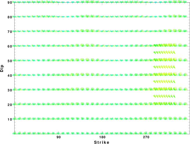
| Focal mechanism sensitivity at the preferred depth. The red color indicates a very good fit to thewavefroms. Each solution is plotted as a vector at a given value of strike and dip with the angle of the vector representing the rake angle, measured, with respect to the upward vertical (N) in the figure. |
A check on the assumed source location is possible by looking at the time shifts between the observed and predicted traces. The time shifts for waveform matching arise for several reasons:
Time_shift = A + B cos Azimuth + C Sin Azimuth
The time shifts for this inversion lead to the next figure:
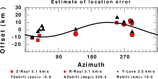
The derived shift in origin time and epicentral coordinates are given at the bottom of the figure.
Should the national backbone of the USGS Advanced National Seismic System (ANSS) be implemented with an interstation separation of 300 km, it is very likely that an earthquake such as this would have been recorded at distances on the order of 100-200 km. This means that the closest station would have information on source depth and mechanism that was lacking here.
Dr. Harley Benz, USGS, provided the USGS USNSN digital data. The digital data used in this study were provided by Natural Resources Canada through their AUTODRM site http://www.seismo.nrcan.gc.ca/nwfa/autodrm/autodrm_req_e.php, and IRIS using their BUD interface.
Thanks also to the many seismic network operators whose dedication make this effort possible: University of Alaska, University of Washington, Oregon State University, University of Utah, Montana Bureas of Mines, UC Berkely, Caltech, UC San Diego, Saint L ouis University, Universityof Memphis, Lamont Doehrty Earth Observatory, Boston College, the Iris stations and the Transportable Array of EarthScope.
The WUS used for the waveform synthetic seismograms and for the surface wave eigenfunctions and dispersion is as follows:
MODEL.01
Model after     8 iterations
ISOTROPIC
KGS
FLAT EARTH
1-D
CONSTANT VELOCITY
LINE08
LINE09
LINE10
LINE11
      H(KM)   VP(KM/S)   VS(KM/S) RHO(GM/CC)         QP         QS       ETAP       ETAS      FREFP      FREFS
     1.9000     3.4065     2.0089     2.2150  0.302E-02  0.679E-02   0.00       0.00       1.00       1.00
     6.1000     5.5445     3.2953     2.6089  0.349E-02  0.784E-02   0.00       0.00       1.00       1.00
    13.0000     6.2708     3.7396     2.7812  0.212E-02  0.476E-02   0.00       0.00       1.00       1.00
    19.0000     6.4075     3.7680     2.8223  0.111E-02  0.249E-02   0.00       0.00       1.00       1.00
     0.0000     7.9000     4.6200     3.2760  0.164E-10  0.370E-10   0.00       0.00       1.00       1.00
Here we tabulate the reasons for not using certain digital data sets
The following stations did not have a valid response files:
DATE=Mon Feb 23 19:49:49 CST 2015