2014/05/31 10:37:20 50.18 12.41 10 4.5 Czech Republic
USGS Felt map for this earthquake
 USGS/SLU Moment Tensor Solution
 ENS  2014/05/31 10:37:20:9  50.18   12.41  10.0 4.5 Czech Republic

 Stations used:
   CH.BALST CH.BERNI CH.BNALP CH.BOURR CH.BRANT CH.DAVOX
   CH.DIX CH.EMBD CH.FIESA CH.FUORN CH.FUSIO CH.GIMEL CH.HASLI
   CH.LAUCH CH.LIENZ CH.LLS CH.MMK CH.MUGIO CH.MUO CH.PANIX
   CH.PLONS CH.SENIN CH.SIMPL CH.SLE CH.TORNY CH.VANNI CH.VDL
   CH.WILA CH.WIMIS CH.ZUR CZ.JAVC CZ.KHC CZ.OKC CZ.PRU
   CZ.PVCC CZ.TREC G.ECH GE.FLT1 GE.IBBN GE.MORC GE.PSZ GE.RUE
   GE.WLF GR.AHRW GR.ASSE GR.BRG GR.BUG GR.CLL GR.CLNZ GR.CLZ
   GR.FUR GR.GEC2 GR.GOLD GR.GRA3 GR.GRB3 GR.GRB5 GR.GRC1
   GR.GRC3 GR.GRC4 GR.GTTG GR.KAST GR.MOX GR.NRDL GR.TMO22
   GR.TNS GR.UBBA GR.UBR GR.WET GR.ZARR GU.CIRO GU.LSD GU.REMY
   HU.BEHE HU.MORH HU.SOP II.BFO IV.BRMO IV.ROVR PL.BEL PL.KSP
   PL.NIE PL.OJC SX.MULD SX.TRIB SX.WIMM TH.ABG1 TH.BBWF
   TH.CRUX TH.GRZ1 TH.HKWD TH.HWTS TH.LEIB1 TH.MLFH TH.MODW
   TH.PLN TH.POSS TH.ZEITZ TH.ZEU

 Filtering commands used:
   cut o DIST/3.3 -40 o DIST/3.3 +70
   rtr
   taper w 0.1
   hp c 0.02 n 3
   lp c 0.06 n 3

 Best Fitting Double Couple
  Mo = 5.89e+21 dyne-cm
  Mw = 3.78
  Z  = 14 km
  Plane   Strike  Dip  Rake
   NP1       35    60    45
   NP2      278    52   141
  Principal Axes:
   Axis    Value   Plunge  Azimuth
    T   5.89e+21     52     251
    N   0.00e+00     38      62
    P  -5.89e+21      5     155

 Moment Tensor: (dyne-cm)
    Component   Value
       Mxx    -4.57e+21
       Mxy     2.93e+21
       Mxz    -5.11e+20
       Myy     9.69e+20
       Myz    -2.90e+21
       Mzz     3.61e+21


                     --------------
                 ----------------------
              --------------------------##
             ---------------------------###
           -----------------------------#####
          ------------------------------######
         -------##################------#######
        ----####################################
        -##############################---######
       ###############################------#####
       ##############################---------###
       ###########   ###############-----------##
       ########### T ##############-------------#
        ##########   #############--------------
        #########################---------------
         ######################----------------
          ###################-----------------
           ################------------------
             ############------------------
              #######--------------   ----
                 ------------------ P -
                     --------------


 Global CMT Convention Moment Tensor:
      R          T          P
  3.61e+21  -5.11e+20   2.90e+21
 -5.11e+20  -4.57e+21  -2.93e+21
  2.90e+21  -2.93e+21   9.69e+20


Details of the solution is found at

http://www.eas.slu.edu/eqc/eqc_mt/MECH.EU/20140531103720/index.html
|
      STK = 35
      DIP = 60
     RAKE = 45
       MW = 3.78
       HS = 14.0
The NDK file is 20140531103720.ndk The waveform inversion is preferred.
The following compares this source inversion to others
 USGS/SLU Moment Tensor Solution
 ENS  2014/05/31 10:37:20:9  50.18   12.41  10.0 4.5 Czech Republic

 Stations used:
   CH.BALST CH.BERNI CH.BNALP CH.BOURR CH.BRANT CH.DAVOX
   CH.DIX CH.EMBD CH.FIESA CH.FUORN CH.FUSIO CH.GIMEL CH.HASLI
   CH.LAUCH CH.LIENZ CH.LLS CH.MMK CH.MUGIO CH.MUO CH.PANIX
   CH.PLONS CH.SENIN CH.SIMPL CH.SLE CH.TORNY CH.VANNI CH.VDL
   CH.WILA CH.WIMIS CH.ZUR CZ.JAVC CZ.KHC CZ.OKC CZ.PRU
   CZ.PVCC CZ.TREC G.ECH GE.FLT1 GE.IBBN GE.MORC GE.PSZ GE.RUE
   GE.WLF GR.AHRW GR.ASSE GR.BRG GR.BUG GR.CLL GR.CLNZ GR.CLZ
   GR.FUR GR.GEC2 GR.GOLD GR.GRA3 GR.GRB3 GR.GRB5 GR.GRC1
   GR.GRC3 GR.GRC4 GR.GTTG GR.KAST GR.MOX GR.NRDL GR.TMO22
   GR.TNS GR.UBBA GR.UBR GR.WET GR.ZARR GU.CIRO GU.LSD GU.REMY
   HU.BEHE HU.MORH HU.SOP II.BFO IV.BRMO IV.ROVR PL.BEL PL.KSP
   PL.NIE PL.OJC SX.MULD SX.TRIB SX.WIMM TH.ABG1 TH.BBWF
   TH.CRUX TH.GRZ1 TH.HKWD TH.HWTS TH.LEIB1 TH.MLFH TH.MODW
   TH.PLN TH.POSS TH.ZEITZ TH.ZEU

 Filtering commands used:
   cut o DIST/3.3 -40 o DIST/3.3 +70
   rtr
   taper w 0.1
   hp c 0.02 n 3
   lp c 0.06 n 3

 Best Fitting Double Couple
  Mo = 5.89e+21 dyne-cm
  Mw = 3.78
  Z  = 14 km
  Plane   Strike  Dip  Rake
   NP1       35    60    45
   NP2      278    52   141
  Principal Axes:
   Axis    Value   Plunge  Azimuth
    T   5.89e+21     52     251
    N   0.00e+00     38      62
    P  -5.89e+21      5     155

 Moment Tensor: (dyne-cm)
    Component   Value
       Mxx    -4.57e+21
       Mxy     2.93e+21
       Mxz    -5.11e+20
       Myy     9.69e+20
       Myz    -2.90e+21
       Mzz     3.61e+21


                     --------------
                 ----------------------
              --------------------------##
             ---------------------------###
           -----------------------------#####
          ------------------------------######
         -------##################------#######
        ----####################################
        -##############################---######
       ###############################------#####
       ##############################---------###
       ###########   ###############-----------##
       ########### T ##############-------------#
        ##########   #############--------------
        #########################---------------
         ######################----------------
          ###################-----------------
           ################------------------
             ############------------------
              #######--------------   ----
                 ------------------ P -
                     --------------


 Global CMT Convention Moment Tensor:
      R          T          P
  3.61e+21  -5.11e+20   2.90e+21
 -5.11e+20  -4.57e+21  -2.93e+21
  2.90e+21  -2.93e+21   9.69e+20


Details of the solution is found at

http://www.eas.slu.edu/eqc/eqc_mt/MECH.EU/20140531103720/index.html
|
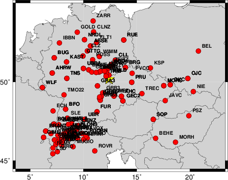
The focal mechanism was determined using broadband seismic waveforms. The location of the event and the and stations used for the waveform inversion are shown in the next figure.
|
|
|
|
The program wvfgrd96 was used with good traces observed at short distance to determine the focal mechanism, depth and seismic moment. This technique requires a high quality signal and well determined velocity model for the Green functions. To the extent that these are the quality data, this type of mechanism should be preferred over the radiation pattern technique which requires the separate step of defining the pressure and tension quadrants and the correct strike.
The observed and predicted traces are filtered using the following gsac commands:
cut o DIST/3.3 -40 o DIST/3.3 +70
rtr
taper w 0.1
hp c 0.02 n 3
lp c 0.06 n 3
The results of this grid search from 0.5 to 19 km depth are as follow:
           DEPTH  STK   DIP  RAKE   MW    FIT
WVFGRD96    1.0    15    90    -5   3.41 0.3316
WVFGRD96    2.0    10    75   -15   3.52 0.3731
WVFGRD96    3.0   190    65   -35   3.60 0.3789
WVFGRD96    4.0   185    55   -35   3.63 0.4013
WVFGRD96    5.0   190    75   -60   3.67 0.4300
WVFGRD96    6.0   185    70   -60   3.69 0.4610
WVFGRD96    7.0   180    65   -65   3.70 0.4832
WVFGRD96    8.0   175    65   -70   3.78 0.5032
WVFGRD96    9.0   170    60   -75   3.79 0.5147
WVFGRD96   10.0    35    60    50   3.74 0.5341
WVFGRD96   11.0    35    60    45   3.76 0.5633
WVFGRD96   12.0    35    60    45   3.77 0.5812
WVFGRD96   13.0    35    60    45   3.77 0.5903
WVFGRD96   14.0    35    60    45   3.78 0.5921
WVFGRD96   15.0    35    60    40   3.78 0.5888
WVFGRD96   16.0    35    60    40   3.79 0.5820
WVFGRD96   17.0    30    65    35   3.80 0.5740
WVFGRD96   18.0    35    65    35   3.80 0.5642
WVFGRD96   19.0    35    65    35   3.80 0.5525
WVFGRD96   20.0    30    70    30   3.81 0.5400
WVFGRD96   21.0    30    70    35   3.81 0.5277
WVFGRD96   22.0    30    70    30   3.82 0.5132
WVFGRD96   23.0    30    70    30   3.83 0.4982
WVFGRD96   24.0    30    70    30   3.83 0.4826
WVFGRD96   25.0    30    70    30   3.83 0.4667
WVFGRD96   26.0    25    75    30   3.84 0.4515
WVFGRD96   27.0    30    75    30   3.84 0.4368
WVFGRD96   28.0    25    75    25   3.85 0.4233
WVFGRD96   29.0    25    75    25   3.85 0.4121
The best solution is
WVFGRD96 14.0 35 60 45 3.78 0.5921
The mechanism correspond to the best fit is
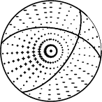
|
|
|
The best fit as a function of depth is given in the following figure:
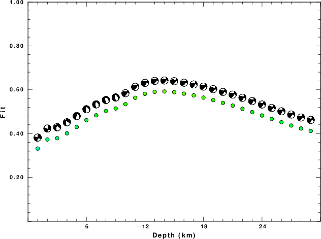
|
|
|
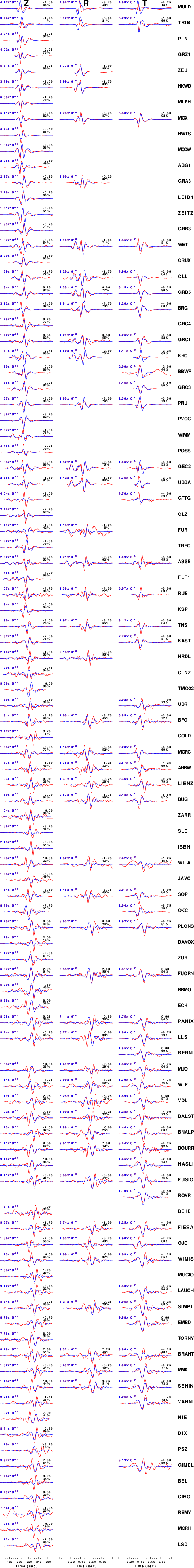
The comparison of the observed and predicted waveforms is given in the next figure. The red traces are the observed and the blue are the predicted. Each observed-predicted component is plotted to the same scale and peak amplitudes are indicated by the numbers to the left of each trace. A pair of numbers is given in black at the right of each predicted traces. The upper number it the time shift required for maximum correlation between the observed and predicted traces. This time shift is required because the synthetics are not computed at exactly the same distance as the observed and because the velocity model used in the predictions may not be perfect. A positive time shift indicates that the prediction is too fast and should be delayed to match the observed trace (shift to the right in this figure). A negative value indicates that the prediction is too slow. The lower number gives the percentage of variance reduction to characterize the individual goodness of fit (100% indicates a perfect fit).
The bandpass filter used in the processing and for the display was
cut o DIST/3.3 -40 o DIST/3.3 +70
rtr
taper w 0.1
hp c 0.02 n 3
lp c 0.06 n 3
|
|
|
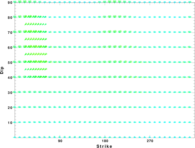
|
| Focal mechanism sensitivity at the preferred depth. The red color indicates a very good fit to thewavefroms. Each solution is plotted as a vector at a given value of strike and dip with the angle of the vector representing the rake angle, measured, with respect to the upward vertical (N) in the figure. |
A check on the assumed source location is possible by looking at the time shifts between the observed and predicted traces. The time shifts for waveform matching arise for several reasons:
Time_shift = A + B cos Azimuth + C Sin Azimuth
The time shifts for this inversion lead to the next figure:
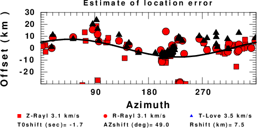
The derived shift in origin time and epicentral coordinates are given at the bottom of the figure.
Should the national backbone of the USGS Advanced National Seismic System (ANSS) be implemented with an interstation separation of 300 km, it is very likely that an earthquake such as this would have been recorded at distances on the order of 100-200 km. This means that the closest station would have information on source depth and mechanism that was lacking here.
Dr. Harley Benz, USGS, provided the USGS USNSN digital data. The digital data used in this study were provided by Natural Resources Canada through their AUTODRM site http://www.seismo.nrcan.gc.ca/nwfa/autodrm/autodrm_req_e.php, and IRIS using their BUD interface.
Thanks also to the many seismic network operators whose dedication make this effort possible: University of Alaska, University of Washington, Oregon State University, University of Utah, Montana Bureas of Mines, UC Berkely, Caltech, UC San Diego, Saint L ouis University, Universityof Memphis, Lamont Doehrty Earth Observatory, Boston College, the Iris stations and the Transportable Array of EarthScope.
The WUS used for the waveform synthetic seismograms and for the surface wave eigenfunctions and dispersion is as follows:
MODEL.01
Model after     8 iterations
ISOTROPIC
KGS
FLAT EARTH
1-D
CONSTANT VELOCITY
LINE08
LINE09
LINE10
LINE11
      H(KM)   VP(KM/S)   VS(KM/S) RHO(GM/CC)         QP         QS       ETAP       ETAS      FREFP      FREFS
     1.9000     3.4065     2.0089     2.2150  0.302E-02  0.679E-02   0.00       0.00       1.00       1.00
     6.1000     5.5445     3.2953     2.6089  0.349E-02  0.784E-02   0.00       0.00       1.00       1.00
    13.0000     6.2708     3.7396     2.7812  0.212E-02  0.476E-02   0.00       0.00       1.00       1.00
    19.0000     6.4075     3.7680     2.8223  0.111E-02  0.249E-02   0.00       0.00       1.00       1.00
     0.0000     7.9000     4.6200     3.2760  0.164E-10  0.370E-10   0.00       0.00       1.00       1.00
Here we tabulate the reasons for not using certain digital data sets
The following stations did not have a valid response files:
DATE=Sat May 31 15:44:14 CDT 2014