Location
2013/07/02 10:45:22 40.12 21.86 7.0 4.7 Greece
Arrival Times (from USGS)
Arrival time list
Felt Map
USGS Felt map for this earthquake
USGS Felt reports archive
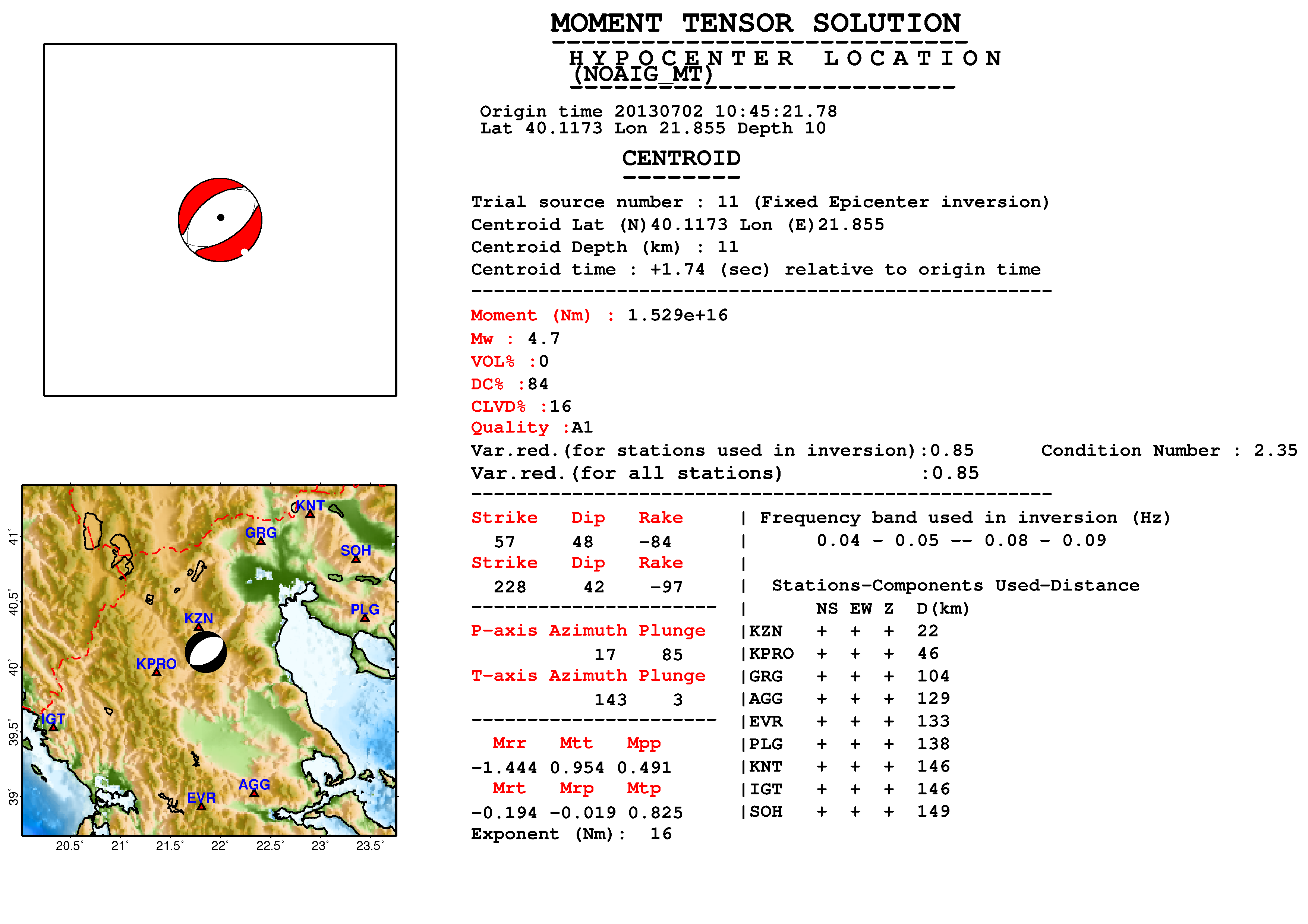
Focal Mechanism
 USGS/SLU Moment Tensor Solution
 ENS  2013/07/02 10:45:22:0  40.12   21.86   7.0 4.7 Greece

 Stations used:
   BS.PLD GE.KTHA HL.APE HL.IMMV HL.KEK HT.AGG HT.ALN HT.GRG
   HT.KNT HT.LIT HT.SIGR HT.SOH HT.THE HT.XOR MN.VTS SJ.BBLS

 Filtering commands used:
   cut a -10 a 150
   rtr
   taper w 0.1
   hp c 0.02 n 3
   lp c 0.06 n 3

 Best Fitting Double Couple
  Mo = 1.68e+23 dyne-cm
  Mw = 4.75
  Z  = 13 km
  Plane   Strike  Dip  Rake
   NP1      226    46   -100
   NP2       60    45   -80
  Principal Axes:
   Axis    Value   Plunge  Azimuth
    T   1.68e+23      0     323
    N   0.00e+00      7     233
    P  -1.68e+23     83      56

 Moment Tensor: (dyne-cm)
    Component   Value
       Mxx     1.06e+23
       Mxy    -8.19e+22
       Mxz    -1.03e+22
       Myy     5.92e+22
       Myz    -1.79e+22
       Mzz    -1.65e+23


                     ##############
                 ######################
              T ##########################
                ##############-------------
           ###############-------------------
          #############-----------------------
         ############-------------------------#
        ###########---------------------------##
        #########----------------------------###
       #########------------   --------------####
       ########------------- P -------------#####
       #######--------------   ------------######
       ######-----------------------------#######
        #####---------------------------########
        #####-------------------------##########
         ###------------------------###########
          ##---------------------#############
           ------------------################
             ##############################
              ############################
                 ######################
                     ##############


 Global CMT Convention Moment Tensor:
      R          T          P
 -1.65e+23  -1.03e+22   1.79e+22
 -1.03e+22   1.06e+23   8.19e+22
  1.79e+22   8.19e+22   5.92e+22


Details of the solution is found at

http://www.eas.slu.edu/eqc/eqc_mt/MECH.EU/20130702104522/index.html
|
Preferred Solution
The preferred solution from an analysis of the surface-wave spectral amplitude radiation pattern, waveform inversion and first motion observations is
      STK = 60
      DIP = 45
     RAKE = -80
       MW = 4.75
       HS = 13.0
The waveform inversion is preferred.
Moment Tensor Comparison
The following compares this source inversion to others
| SLU |
NOAIG |
 USGS/SLU Moment Tensor Solution
 ENS  2013/07/02 10:45:22:0  40.12   21.86   7.0 4.7 Greece

 Stations used:
   BS.PLD GE.KTHA HL.APE HL.IMMV HL.KEK HT.AGG HT.ALN HT.GRG
   HT.KNT HT.LIT HT.SIGR HT.SOH HT.THE HT.XOR MN.VTS SJ.BBLS

 Filtering commands used:
   cut a -10 a 150
   rtr
   taper w 0.1
   hp c 0.02 n 3
   lp c 0.06 n 3

 Best Fitting Double Couple
  Mo = 1.68e+23 dyne-cm
  Mw = 4.75
  Z  = 13 km
  Plane   Strike  Dip  Rake
   NP1      226    46   -100
   NP2       60    45   -80
  Principal Axes:
   Axis    Value   Plunge  Azimuth
    T   1.68e+23      0     323
    N   0.00e+00      7     233
    P  -1.68e+23     83      56

 Moment Tensor: (dyne-cm)
    Component   Value
       Mxx     1.06e+23
       Mxy    -8.19e+22
       Mxz    -1.03e+22
       Myy     5.92e+22
       Myz    -1.79e+22
       Mzz    -1.65e+23


                     ##############
                 ######################
              T ##########################
                ##############-------------
           ###############-------------------
          #############-----------------------
         ############-------------------------#
        ###########---------------------------##
        #########----------------------------###
       #########------------   --------------####
       ########------------- P -------------#####
       #######--------------   ------------######
       ######-----------------------------#######
        #####---------------------------########
        #####-------------------------##########
         ###------------------------###########
          ##---------------------#############
           ------------------################
             ##############################
              ############################
                 ######################
                     ##############


 Global CMT Convention Moment Tensor:
      R          T          P
 -1.65e+23  -1.03e+22   1.79e+22
 -1.03e+22   1.06e+23   8.19e+22
  1.79e+22   8.19e+22   5.92e+22


Details of the solution is found at

http://www.eas.slu.edu/eqc/eqc_mt/MECH.EU/20130702104522/index.html
|
|
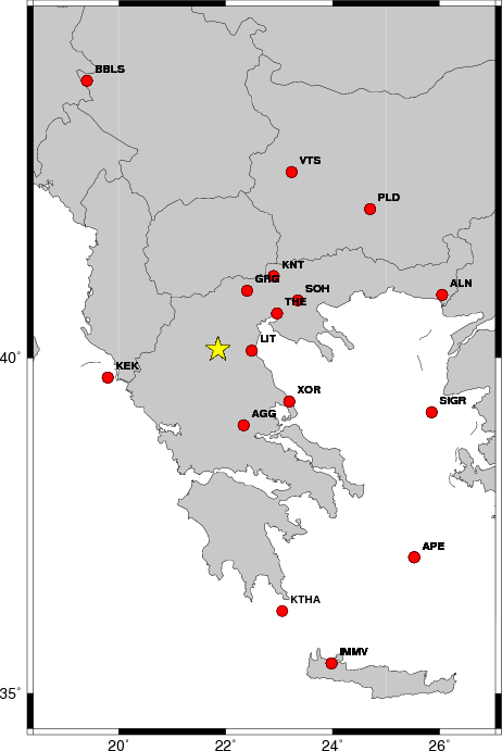
Waveform Inversion
The focal mechanism was determined using broadband seismic waveforms. The location of the event and the
and stations used for the waveform inversion are shown in the next figure.
|
|
Location of broadband stations used for waveform inversion
|
The program wvfgrd96 was used with good traces observed at short distance to determine the focal mechanism, depth and seismic moment. This technique requires a high quality signal and well determined velocity model for the Green functions. To the extent that these are the quality data, this type of mechanism should be preferred over the radiation pattern technique which requires the separate step of defining the pressure and tension quadrants and the correct strike.
The observed and predicted traces are filtered using the following gsac commands:
cut a -10 a 150
rtr
taper w 0.1
hp c 0.02 n 3
lp c 0.06 n 3
The results of this grid search from 0.5 to 19 km depth are as follow:
           DEPTH  STK   DIP  RAKE   MW    FIT
WVFGRD96    0.5   225    45  -100   4.35 0.2641
WVFGRD96    1.0   100    90     0   4.27 0.2674
WVFGRD96    2.0   280    85    -5   4.38 0.3400
WVFGRD96    3.0   275    60   -10   4.46 0.3687
WVFGRD96    4.0   275    55   -10   4.51 0.4003
WVFGRD96    5.0   275    55   -10   4.54 0.4274
WVFGRD96    6.0   275    55   -10   4.56 0.4527
WVFGRD96    7.0   275    55   -10   4.57 0.4777
WVFGRD96    8.0   265    65   -45   4.65 0.5065
WVFGRD96    9.0   255    60   -60   4.70 0.5438
WVFGRD96   10.0    50    40   -95   4.74 0.5902
WVFGRD96   11.0    55    40   -85   4.75 0.6209
WVFGRD96   12.0    60    45   -80   4.75 0.6387
WVFGRD96   13.0    60    45   -80   4.75 0.6457
WVFGRD96   14.0    65    45   -70   4.75 0.6452
WVFGRD96   15.0    65    45   -70   4.75 0.6417
WVFGRD96   16.0    70    45   -65   4.75 0.6351
WVFGRD96   17.0    75    50   -55   4.74 0.6290
WVFGRD96   18.0    75    50   -55   4.75 0.6214
WVFGRD96   19.0    80    55   -45   4.75 0.6145
WVFGRD96   20.0    85    55   -40   4.75 0.6071
WVFGRD96   21.0    85    55   -40   4.77 0.6057
WVFGRD96   22.0    85    60   -35   4.77 0.5982
WVFGRD96   23.0    85    60   -35   4.78 0.5909
WVFGRD96   24.0    85    60   -35   4.79 0.5827
WVFGRD96   25.0    85    60   -35   4.79 0.5736
WVFGRD96   26.0    85    60   -35   4.80 0.5638
WVFGRD96   27.0    85    60   -35   4.80 0.5538
WVFGRD96   28.0    85    60   -35   4.81 0.5429
WVFGRD96   29.0    90    65   -30   4.82 0.5320
The best solution is
WVFGRD96 13.0 60 45 -80 4.75 0.6457
The mechanism correspond to the best fit is
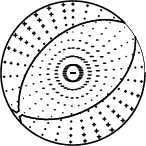
|
|
Figure 1. Waveform inversion focal mechanism
|
The best fit as a function of depth is given in the following figure:
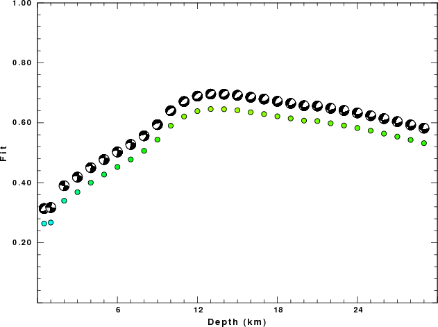
|
|
Figure 2. Depth sensitivity for waveform mechanism
|
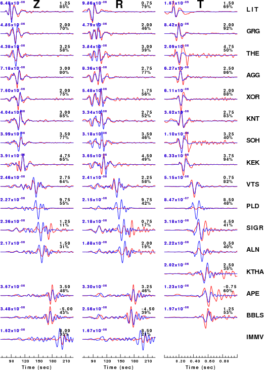
The comparison of the observed and predicted waveforms is given in the next figure. The red traces are the observed and the blue are the predicted.
Each observed-predicted component is plotted to the same scale and peak amplitudes are indicated by the numbers to the left of each trace. A pair of numbers is given in black at the right of each predicted traces. The upper number it the time shift required for maximum correlation between the observed and predicted traces. This time shift is required because the synthetics are not computed at exactly the same distance as the observed and because the velocity model used in the predictions may not be perfect.
A positive time shift indicates that the prediction is too fast and should be delayed to match the observed trace (shift to the right in this figure). A negative value indicates that the prediction is too slow. The lower number gives the percentage of variance reduction to characterize the individual goodness of fit (100% indicates a perfect fit).
The bandpass filter used in the processing and for the display was
cut a -10 a 150
rtr
taper w 0.1
hp c 0.02 n 3
lp c 0.06 n 3
|
|
Figure 3. Waveform comparison for selected depth. Red: observed; Blue - predicted. The time shift with respect to the model prediction is indicated. The percent of fit is also indicated.
|
|
|
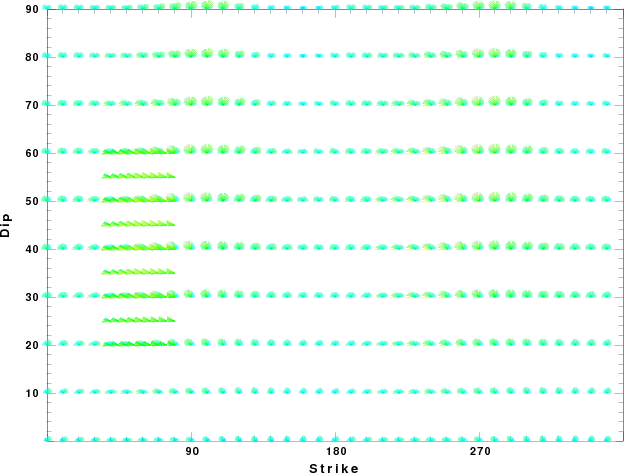
Focal mechanism sensitivity at the preferred depth. The red color indicates a very good fit to thewavefroms.
Each solution is plotted as a vector at a given value of strike and dip with the angle of the vector representing the rake angle, measured, with respect to the upward vertical (N) in the figure.
|
A check on the assumed source location is possible by looking at the time shifts between the observed and predicted traces. The time shifts for waveform matching arise for several reasons:
- The origin time and epicentral distance are incorrect
- The velocity model used for the inversion is incorrect
- The velocity model used to define the P-arrival time is not the
same as the velocity model used for the waveform inversion
(assuming that the initial trace alignment is based on the
P arrival time)
Assuming only a mislocation, the time shifts are fit to a functional form:
Time_shift = A + B cos Azimuth + C Sin Azimuth
The time shifts for this inversion lead to the next figure:
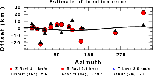
The derived shift in origin time and epicentral coordinates are given at the bottom of the figure.
Discussion
The Future
Should the national backbone of the
USGS Advanced National Seismic System (ANSS)
be implemented with an interstation separation of 300 km, it is very likely that
an earthquake such as this would have been recorded at distances on the order of
100-200 km. This means that the closest station would have information on
source depth and mechanism that was lacking here.
Acknowledgements
Dr. Harley Benz, USGS, provided the USGS USNSN digital data.
The digital data used in this study were provided by Natural Resources Canada through their AUTODRM site http://www.seismo.nrcan.gc.ca/nwfa/autodrm/autodrm_req_e.php, and IRIS using their BUD interface.
Thanks also to the many seismic network operators whose dedication make this effort possible: University of Alaska, University of Washington, Oregon State University, University of Utah, Montana Bureas of Mines, UC Berkely, Caltech, UC San Diego, Saint L ouis University, Universityof Memphis, Lamont Doehrty Earth Observatory, Boston College, the Iris stations and the Transportable Array of EarthScope.
Velocity Model
The WUS used for the waveform synthetic seismograms and for the surface wave eigenfunctions and dispersion is as follows:
MODEL.01
Model after     8 iterations
ISOTROPIC
KGS
FLAT EARTH
1-D
CONSTANT VELOCITY
LINE08
LINE09
LINE10
LINE11
      H(KM)   VP(KM/S)   VS(KM/S) RHO(GM/CC)         QP         QS       ETAP       ETAS      FREFP      FREFS
     1.9000     3.4065     2.0089     2.2150  0.302E-02  0.679E-02   0.00       0.00       1.00       1.00
     6.1000     5.5445     3.2953     2.6089  0.349E-02  0.784E-02   0.00       0.00       1.00       1.00
    13.0000     6.2708     3.7396     2.7812  0.212E-02  0.476E-02   0.00       0.00       1.00       1.00
    19.0000     6.4075     3.7680     2.8223  0.111E-02  0.249E-02   0.00       0.00       1.00       1.00
     0.0000     7.9000     4.6200     3.2760  0.164E-10  0.370E-10   0.00       0.00       1.00       1.00
Quality Control
Here we tabulate the reasons for not using certain digital data sets
The following stations did not have a valid response files:
DATE=Tue Jul 2 09:06:19 CDT 2013
Last Changed 2013/07/02