Location
2013/06/16 20:05:00 45.79 14.87 10.0 4.10 Slovenia
Arrival Times (from USGS)
Arrival time list
Felt Map
USGS Felt map for this earthquake
USGS Felt reports archive
Focal Mechanism
 USGS/SLU Moment Tensor Solution
 ENS  2013/06/16 20:05:00:1  45.79   14.87  10.0 4.1 Slovenia

 Stations used:
   CZ.JAVC CZ.KHC CZ.KRUC CZ.PRU CZ.TREC CZ.VRAC GE.MORC
   GE.PSZ GR.BRG GR.CLL GR.FUR GR.GEC2 GR.GRB1 GR.GRB3 GR.MOX
   GR.UBBA GR.UBR GR.WET HU.BEHE HU.BUD HU.SOP IV.PTCC IV.STAL
   MN.BLY MN.PDG MN.TIR MN.TRI MN.TUE NI.ACOM NI.CGRP NI.SABO
   OE.ABTA OE.ARSA OE.CONA OE.CSNA OE.DAVA OE.FETA OE.KBA
   OE.MOA OE.MYKA OE.OBKA OE.RETA OE.SOKA OE.WTTA PL.KSP
   SJ.BBLS SJ.FRGS SX.TANN TH.HKWD TH.HWTS TH.MODW

 Filtering commands used:
   hp c 0.02 n 3
   lp c 0.06 n 3

 Best Fitting Double Couple
  Mo = 5.50e+21 dyne-cm
  Mw = 3.76
  Z  = 15 km
  Plane   Strike  Dip  Rake
   NP1      143    69   -148
   NP2       40    60   -25
  Principal Axes:
   Axis    Value   Plunge  Azimuth
    T   5.50e+21      5     270
    N   0.00e+00     52     173
    P  -5.50e+21     38       4

 Moment Tensor: (dyne-cm)
    Component   Value
       Mxx    -3.42e+21
       Mxy    -2.41e+20
       Mxz    -2.65e+21
       Myy     5.43e+21
       Myz    -7.11e+20
       Mzz    -2.01e+21


                     --------------
                 ----------------------
              ##-------------------------#
             ###-----------   ------------#
           #####----------- P -----------####
          #######----------   -----------#####
         ########------------------------######
        ##########----------------------########
        ###########---------------------########
       #############-------------------##########
          ###########-----------------###########
        T ############---------------############
          #############------------##############
        #################---------##############
        ##################------################
         ###################---################
          ##################--################
           ###############------#############
             ##########------------########
              ###---------------------####
                 ----------------------
                     --------------


 Global CMT Convention Moment Tensor:
      R          T          P
 -2.01e+21  -2.65e+21   7.11e+20
 -2.65e+21  -3.42e+21   2.41e+20
  7.11e+20   2.41e+20   5.43e+21


Details of the solution is found at

http://www.eas.slu.edu/eqc/eqc_mt/MECH.EU/20130616200500/index.html
|
Preferred Solution
The preferred solution from an analysis of the surface-wave spectral amplitude radiation pattern, waveform inversion and first motion observations is
      STK = 40
      DIP = 60
     RAKE = -25
       MW = 3.76
       HS = 15.0
The NDK file is 20130616200500.ndk.
The waveform inversion is preferred.
Moment Tensor Comparison
The following compares this source inversion to others
| SLU |
OGS |
 USGS/SLU Moment Tensor Solution
 ENS  2013/06/16 20:05:00:1  45.79   14.87  10.0 4.1 Slovenia

 Stations used:
   CZ.JAVC CZ.KHC CZ.KRUC CZ.PRU CZ.TREC CZ.VRAC GE.MORC
   GE.PSZ GR.BRG GR.CLL GR.FUR GR.GEC2 GR.GRB1 GR.GRB3 GR.MOX
   GR.UBBA GR.UBR GR.WET HU.BEHE HU.BUD HU.SOP IV.PTCC IV.STAL
   MN.BLY MN.PDG MN.TIR MN.TRI MN.TUE NI.ACOM NI.CGRP NI.SABO
   OE.ABTA OE.ARSA OE.CONA OE.CSNA OE.DAVA OE.FETA OE.KBA
   OE.MOA OE.MYKA OE.OBKA OE.RETA OE.SOKA OE.WTTA PL.KSP
   SJ.BBLS SJ.FRGS SX.TANN TH.HKWD TH.HWTS TH.MODW

 Filtering commands used:
   hp c 0.02 n 3
   lp c 0.06 n 3

 Best Fitting Double Couple
  Mo = 5.50e+21 dyne-cm
  Mw = 3.76
  Z  = 15 km
  Plane   Strike  Dip  Rake
   NP1      143    69   -148
   NP2       40    60   -25
  Principal Axes:
   Axis    Value   Plunge  Azimuth
    T   5.50e+21      5     270
    N   0.00e+00     52     173
    P  -5.50e+21     38       4

 Moment Tensor: (dyne-cm)
    Component   Value
       Mxx    -3.42e+21
       Mxy    -2.41e+20
       Mxz    -2.65e+21
       Myy     5.43e+21
       Myz    -7.11e+20
       Mzz    -2.01e+21


                     --------------
                 ----------------------
              ##-------------------------#
             ###-----------   ------------#
           #####----------- P -----------####
          #######----------   -----------#####
         ########------------------------######
        ##########----------------------########
        ###########---------------------########
       #############-------------------##########
          ###########-----------------###########
        T ############---------------############
          #############------------##############
        #################---------##############
        ##################------################
         ###################---################
          ##################--################
           ###############------#############
             ##########------------########
              ###---------------------####
                 ----------------------
                     --------------


 Global CMT Convention Moment Tensor:
      R          T          P
 -2.01e+21  -2.65e+21   7.11e+20
 -2.65e+21  -3.42e+21   2.41e+20
  7.11e+20   2.41e+20   5.43e+21


Details of the solution is found at

http://www.eas.slu.edu/eqc/eqc_mt/MECH.EU/20130616200500/index.html
|
Centro Ricerche Sismologiche
Istituto Nazionale di Oceanografia e Geofisica Sperimentale - OGS
 MT Site
|
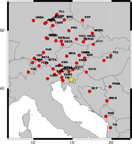
Waveform Inversion
The focal mechanism was determined using broadband seismic waveforms. The location of the event and the
and stations used for the waveform inversion are shown in the next figure.
|
|
Location of broadband stations used for waveform inversion
|
The program wvfgrd96 was used with good traces observed at short distance to determine the focal mechanism, depth and seismic moment. This technique requires a high quality signal and well determined velocity model for the Green functions. To the extent that these are the quality data, this type of mechanism should be preferred over the radiation pattern technique which requires the separate step of defining the pressure and tension quadrants and the correct strike.
The observed and predicted traces are filtered using the following gsac commands:
hp c 0.02 n 3
lp c 0.06 n 3
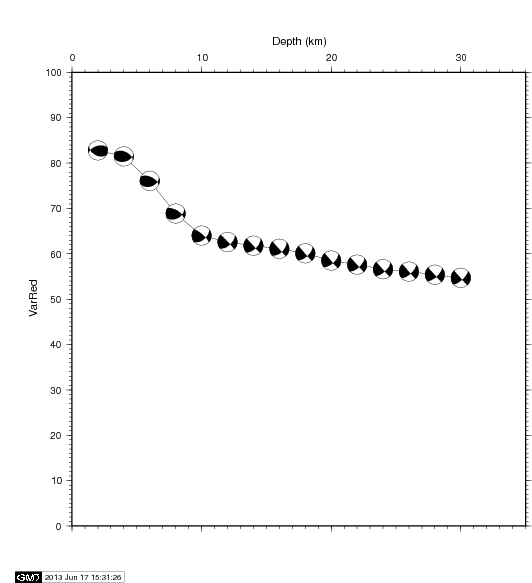
The results of this grid search from 0.5 to 19 km depth are as follow:
           DEPTH  STK   DIP  RAKE   MW    FIT
WVFGRD96    0.5    85    50    90   3.44 0.3838
WVFGRD96    1.0    80    45    85   3.48 0.3863
WVFGRD96    2.0    80    50    80   3.59 0.4743
WVFGRD96    3.0    65    55    55   3.63 0.4883
WVFGRD96    4.0    65    55    55   3.65 0.4809
WVFGRD96    5.0    60    60    45   3.64 0.4533
WVFGRD96    6.0   230    80    40   3.62 0.4555
WVFGRD96    7.0    45    85   -35   3.63 0.4703
WVFGRD96    8.0    45    90   -40   3.67 0.4839
WVFGRD96    9.0    45    85   -40   3.68 0.4945
WVFGRD96   10.0    40    75   -35   3.69 0.5077
WVFGRD96   11.0    40    75   -35   3.70 0.5171
WVFGRD96   12.0    35    55   -30   3.73 0.5248
WVFGRD96   13.0    35    55   -30   3.74 0.5334
WVFGRD96   14.0    40    60   -25   3.75 0.5376
WVFGRD96   15.0    40    60   -25   3.76 0.5393
WVFGRD96   16.0    40    60   -25   3.76 0.5378
WVFGRD96   17.0    40    55   -20   3.77 0.5352
WVFGRD96   18.0    40    55   -20   3.78 0.5317
WVFGRD96   19.0    40    55   -20   3.79 0.5267
WVFGRD96   20.0    40    55   -20   3.79 0.5205
WVFGRD96   21.0    35    50   -20   3.80 0.5124
WVFGRD96   22.0    35    50   -20   3.80 0.5055
WVFGRD96   23.0    35    50   -20   3.81 0.4987
WVFGRD96   24.0    35    50   -15   3.82 0.4919
WVFGRD96   25.0    35    50   -15   3.83 0.4852
WVFGRD96   26.0    35    50   -15   3.83 0.4788
WVFGRD96   27.0    45    40    20   3.85 0.4740
WVFGRD96   28.0    45    45    15   3.86 0.4687
WVFGRD96   29.0    45    45    20   3.86 0.4628
The best solution is
WVFGRD96 15.0 40 60 -25 3.76 0.5393
The mechanism correspond to the best fit is
|
|
Figure 1. Waveform inversion focal mechanism
|
The best fit as a function of depth is given in the following figure:
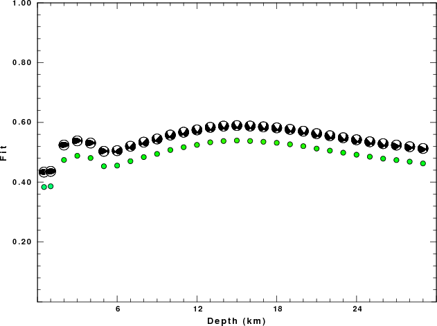
|
|
Figure 2. Depth sensitivity for waveform mechanism
|
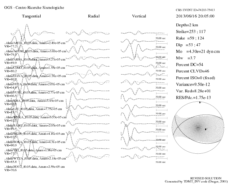
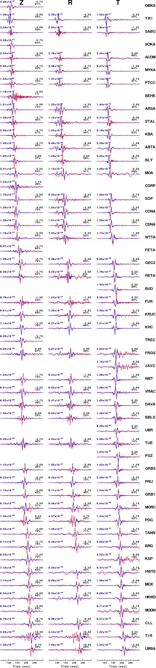
The comparison of the observed and predicted waveforms is given in the next figure. The red traces are the observed and the blue are the predicted.
Each observed-predicted component is plotted to the same scale and peak amplitudes are indicated by the numbers to the left of each trace. A pair of numbers is given in black at the right of each predicted traces. The upper number it the time shift required for maximum correlation between the observed and predicted traces. This time shift is required because the synthetics are not computed at exactly the same distance as the observed and because the velocity model used in the predictions may not be perfect.
A positive time shift indicates that the prediction is too fast and should be delayed to match the observed trace (shift to the right in this figure). A negative value indicates that the prediction is too slow. The lower number gives the percentage of variance reduction to characterize the individual goodness of fit (100% indicates a perfect fit).
The bandpass filter used in the processing and for the display was
hp c 0.02 n 3
lp c 0.06 n 3
|
|
Figure 3. Waveform comparison for selected depth
|
|
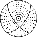
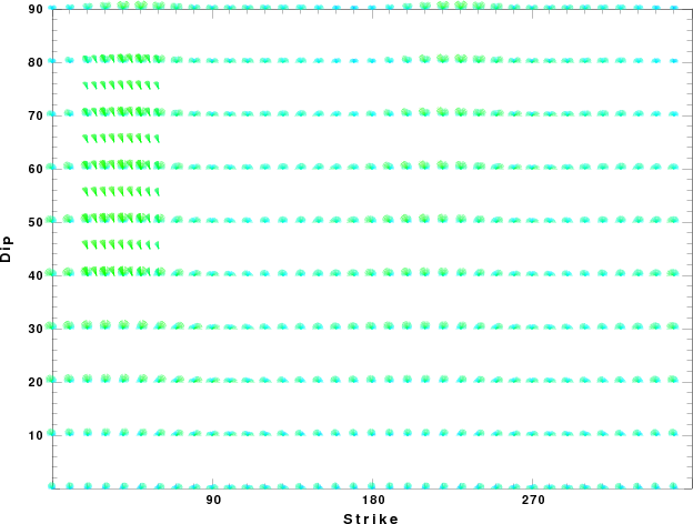
|
Focal mechanism sensitivity at the preferred depth. The red color indicates a very good fit to thewavefroms.
Each solution is plotted as a vector at a given value of strike and dip with the angle of the vector representing the rake angle, measured, with respect to the upward vertical (N) in the figure.
|
A check on the assumed source location is possible by looking at the time shifts between the observed and predicted traces. The time shifts for waveform matching arise for several reasons:
- The origin time and epicentral distance are incorrect
- The velocity model used for the inversion is incorrect
- The velocity model used to define the P-arrival time is not the
same as the velocity model used for the waveform inversion
(assuming that the initial trace alignment is based on the
P arrival time)
Assuming only a mislocation, the time shifts are fit to a functional form:
Time_shift = A + B cos Azimuth + C Sin Azimuth
The time shifts for this inversion lead to the next figure:
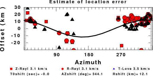
The derived shift in origin time and epicentral coordinates are given at the bottom of the figure.
Discussion
The Future
Should the national backbone of the
USGS Advanced National Seismic System (ANSS)
be implemented with an interstation separation of 300 km, it is very likely that
an earthquake such as this would have been recorded at distances on the order of
100-200 km. This means that the closest station would have information on
source depth and mechanism that was lacking here.
Acknowledgements
Dr. Harley Benz, USGS, provided the USGS USNSN digital data.
The digital data used in this study were provided by Natural Resources Canada through their AUTODRM site http://www.seismo.nrcan.gc.ca/nwfa/autodrm/autodrm_req_e.php, and IRIS using their BUD interface.
Thanks also to the many seismic network operators whose dedication make this effort possible: University of Alaska, University of Washington, Oregon State University, University of Utah, Montana Bureas of Mines, UC Berkely, Caltech, UC San Diego, Saint L ouis University, Universityof Memphis, Lamont Doehrty Earth Observatory, Boston College, the Iris stations and the Transportable Array of EarthScope.
Velocity Model
The WUS used for the waveform synthetic seismograms and for the surface wave eigenfunctions and dispersion is as follows:
MODEL.01
Model after     8 iterations
ISOTROPIC
KGS
FLAT EARTH
1-D
CONSTANT VELOCITY
LINE08
LINE09
LINE10
LINE11
      H(KM)   VP(KM/S)   VS(KM/S) RHO(GM/CC)         QP         QS       ETAP       ETAS      FREFP      FREFS
     1.9000     3.4065     2.0089     2.2150  0.302E-02  0.679E-02   0.00       0.00       1.00       1.00
     6.1000     5.5445     3.2953     2.6089  0.349E-02  0.784E-02   0.00       0.00       1.00       1.00
    13.0000     6.2708     3.7396     2.7812  0.212E-02  0.476E-02   0.00       0.00       1.00       1.00
    19.0000     6.4075     3.7680     2.8223  0.111E-02  0.249E-02   0.00       0.00       1.00       1.00
     0.0000     7.9000     4.6200     3.2760  0.164E-10  0.370E-10   0.00       0.00       1.00       1.00
Quality Control
Here we tabulate the reasons for not using certain digital data sets
The following stations did not have a valid response files:
DATE=Tue Jun 18 02:12:45 CDT 2013
Last Changed 2013/06/16