2011/09/25 13:17:10 42.53 18.57 2.0 4.40 Montenegro
USGS Felt map for this earthquake
 USGS/SLU Moment Tensor Solution
 ENS  2011/09/25 13:17:10:0  42.53   18.57   2.0 4.4 Montenegro

 Stations used:
   HT.GRG HT.HORT HT.SRS HT.THE MN.DIVS MN.PDG MN.TIR MN.VTS
   OE.ABTA OE.ARSA OE.MOA OE.MYKA OE.OBKA OE.SOKA RO.BZS
   SL.BOJS SL.CRES SL.GBAS SL.GCIS SL.KOGS SL.LJU SL.MOZS
   SL.PERS SL.ROBS SL.SKDS SL.VISS

 Filtering commands used:
   hp c 0.02 n 3
   lp c 0.05 n 3

 Best Fitting Double Couple
  Mo = 9.55e+21 dyne-cm
  Mw = 3.92
  Z  = 12 km
  Plane   Strike  Dip  Rake
   NP1      142    69   103
   NP2      290    25    60
  Principal Axes:
   Axis    Value   Plunge  Azimuth
    T   9.55e+21     64      74
    N   0.00e+00     12     318
    P  -9.55e+21     22     222

 Moment Tensor: (dyne-cm)
    Component   Value
       Mxx    -4.30e+21
       Mxy    -3.58e+21
       Mxz     3.52e+21
       Myy    -2.04e+21
       Myz     5.88e+21
       Mzz     6.34e+21


                     --------------
                 ----------------------
              #------#########------------
             #######################-------
           ##---#######################------
          #-----#########################-----
         --------##########################----
        ----------##########################----
        -----------##########################---
       -------------#############   ##########---
       --------------############ T ###########--
       ---------------###########   ###########--
       ----------------#########################-
        -----------------#######################
        ------------------######################
         -------------------###################
          -----   ------------################
           ---- P --------------#############
             --   -----------------########
              ------------------------####
                 ----------------------
                     --------------


 Global CMT Convention Moment Tensor:
      R          T          P
  6.34e+21   3.52e+21  -5.88e+21
  3.52e+21  -4.30e+21   3.58e+21
 -5.88e+21   3.58e+21  -2.04e+21


Details of the solution is found at

http://www.eas.slu.edu/eqc/eqc_mt/MECH.EU/20110925131710/index.html
|
      STK = 290
      DIP = 25
     RAKE = 60
       MW = 3.92
       HS = 12.0
The waveform inversion is preferred.
The following compares this source inversion to others
 USGS/SLU Moment Tensor Solution
 ENS  2011/09/25 13:17:10:0  42.53   18.57   2.0 4.4 Montenegro

 Stations used:
   HT.GRG HT.HORT HT.SRS HT.THE MN.DIVS MN.PDG MN.TIR MN.VTS
   OE.ABTA OE.ARSA OE.MOA OE.MYKA OE.OBKA OE.SOKA RO.BZS
   SL.BOJS SL.CRES SL.GBAS SL.GCIS SL.KOGS SL.LJU SL.MOZS
   SL.PERS SL.ROBS SL.SKDS SL.VISS

 Filtering commands used:
   hp c 0.02 n 3
   lp c 0.05 n 3

 Best Fitting Double Couple
  Mo = 9.55e+21 dyne-cm
  Mw = 3.92
  Z  = 12 km
  Plane   Strike  Dip  Rake
   NP1      142    69   103
   NP2      290    25    60
  Principal Axes:
   Axis    Value   Plunge  Azimuth
    T   9.55e+21     64      74
    N   0.00e+00     12     318
    P  -9.55e+21     22     222

 Moment Tensor: (dyne-cm)
    Component   Value
       Mxx    -4.30e+21
       Mxy    -3.58e+21
       Mxz     3.52e+21
       Myy    -2.04e+21
       Myz     5.88e+21
       Mzz     6.34e+21


                     --------------
                 ----------------------
              #------#########------------
             #######################-------
           ##---#######################------
          #-----#########################-----
         --------##########################----
        ----------##########################----
        -----------##########################---
       -------------#############   ##########---
       --------------############ T ###########--
       ---------------###########   ###########--
       ----------------#########################-
        -----------------#######################
        ------------------######################
         -------------------###################
          -----   ------------################
           ---- P --------------#############
             --   -----------------########
              ------------------------####
                 ----------------------
                     --------------


 Global CMT Convention Moment Tensor:
      R          T          P
  6.34e+21   3.52e+21  -5.88e+21
  3.52e+21  -4.30e+21   3.58e+21
 -5.88e+21   3.58e+21  -2.04e+21


Details of the solution is found at

http://www.eas.slu.edu/eqc/eqc_mt/MECH.EU/20110925131710/index.html
|
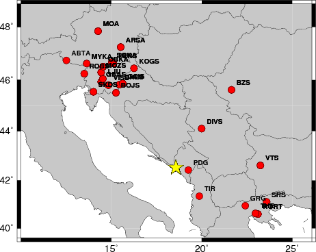
The focal mechanism was determined using broadband seismic waveforms. The location of the event and the and stations used for the waveform inversion are shown in the next figure.
|
|
|
|
The program wvfgrd96 was used with good traces observed at short distance to determine the focal mechanism, depth and seismic moment. This technique requires a high quality signal and well determined velocity model for the Green functions. To the extent that these are the quality data, this type of mechanism should be preferred over the radiation pattern technique which requires the separate step of defining the pressure and tension quadrants and the correct strike.
The observed and predicted traces are filtered using the following gsac commands:
hp c 0.02 n 3
lp c 0.05 n 3
The results of this grid search from 0.5 to 19 km depth are as follow:
           DEPTH  STK   DIP  RAKE   MW    FIT
WVFGRD96    0.5   350    40   100   3.62 0.3932
WVFGRD96    1.0   160    75    10   3.59 0.3675
WVFGRD96    2.0   160    50    85   3.71 0.3805
WVFGRD96    3.0   165    90   -45   3.75 0.3467
WVFGRD96    4.0   280    35    35   3.84 0.3764
WVFGRD96    5.0   285    25    45   3.86 0.4105
WVFGRD96    6.0   285    25    45   3.85 0.4457
WVFGRD96    7.0   290    25    55   3.86 0.4717
WVFGRD96    8.0   290    25    55   3.93 0.5008
WVFGRD96    9.0   290    25    55   3.92 0.5208
WVFGRD96   10.0   295    25    65   3.94 0.5346
WVFGRD96   11.0   290    25    60   3.93 0.5419
WVFGRD96   12.0   290    25    60   3.92 0.5437
WVFGRD96   13.0   290    25    60   3.92 0.5420
WVFGRD96   14.0   280    30    50   3.91 0.5379
WVFGRD96   15.0   280    30    50   3.91 0.5318
WVFGRD96   16.0   280    30    50   3.91 0.5244
WVFGRD96   17.0   275    30    45   3.91 0.5163
WVFGRD96   18.0   275    30    45   3.91 0.5068
WVFGRD96   19.0   270    30    40   3.90 0.4971
WVFGRD96   20.0   270    30    40   3.91 0.4869
WVFGRD96   21.0   270    30    40   3.92 0.4795
WVFGRD96   22.0   265    35    35   3.92 0.4692
WVFGRD96   23.0   265    35    30   3.92 0.4589
WVFGRD96   24.0   265    35    30   3.92 0.4487
WVFGRD96   25.0   265    35    30   3.92 0.4382
WVFGRD96   26.0   265    35    30   3.92 0.4273
WVFGRD96   27.0   260    40    25   3.93 0.4172
WVFGRD96   28.0   260    40    25   3.93 0.4070
WVFGRD96   29.0   260    40    25   3.93 0.3965
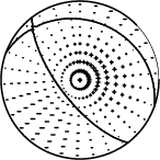
The best solution is
WVFGRD96 12.0 290 25 60 3.92 0.5437
The mechanism correspond to the best fit is
|
|
|
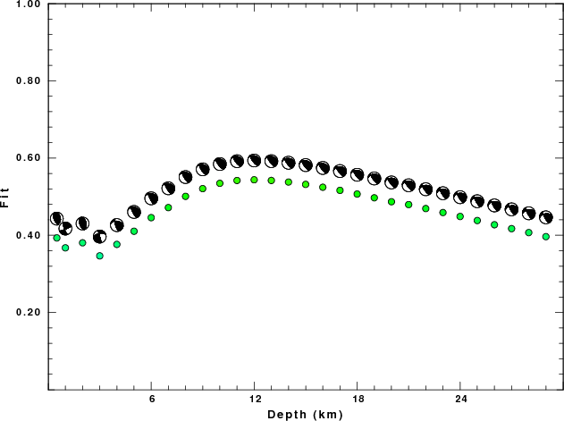
The best fit as a function of depth is given in the following figure:
|
|
|
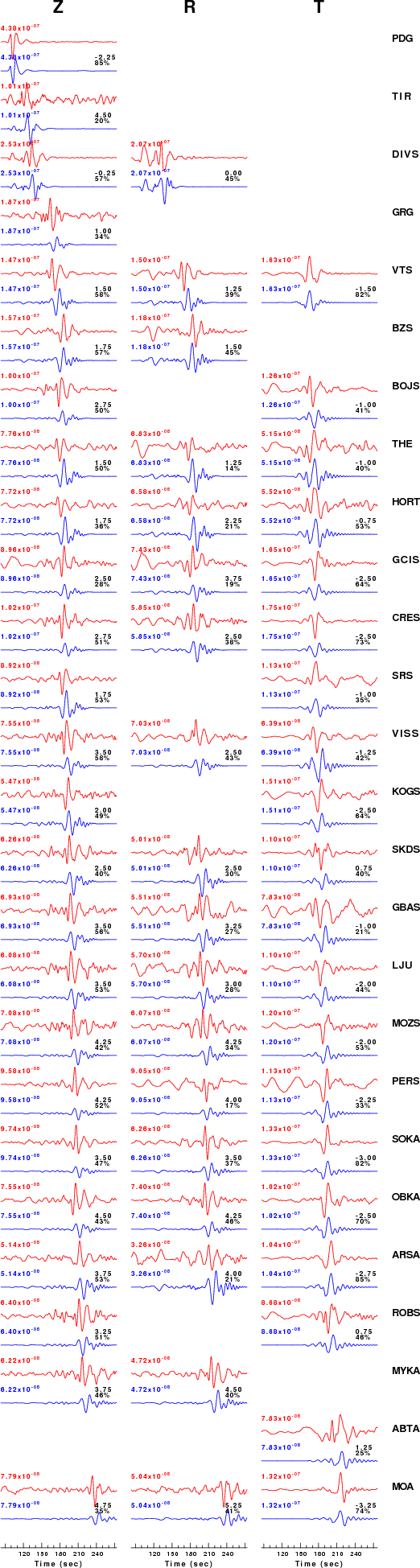
The comparison of the observed and predicted waveforms is given in the next figure. The red traces are the observed and the blue are the predicted. Each observed-predicted component is plotted to the same scale and peak amplitudes are indicated by the numbers to the left of each trace. A pair of numbers is given in black at the right of each predicted traces. The upper number it the time shift required for maximum correlation between the observed and predicted traces. This time shift is required because the synthetics are not computed at exactly the same distance as the observed and because the velocity model used in the predictions may not be perfect. A positive time shift indicates that the prediction is too fast and should be delayed to match the observed trace (shift to the right in this figure). A negative value indicates that the prediction is too slow. The lower number gives the percentage of variance reduction to characterize the individual goodness of fit (100% indicates a perfect fit).
The bandpass filter used in the processing and for the display was
hp c 0.02 n 3
lp c 0.05 n 3
|
|
|
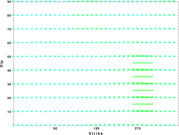
|
| Focal mechanism sensitivity at the preferred depth. The red color indicates a very good fit to thewavefroms. Each solution is plotted as a vector at a given value of strike and dip with the angle of the vector representing the rake angle, measured, with respect to the upward vertical (N) in the figure. |
A check on the assumed source location is possible by looking at the time shifts between the observed and predicted traces. The time shifts for waveform matching arise for several reasons:
Time_shift = A + B cos Azimuth + C Sin Azimuth
The time shifts for this inversion lead to the next figure:
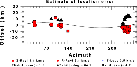
The derived shift in origin time and epicentral coordinates are given at the bottom of the figure.
Should the national backbone of the USGS Advanced National Seismic System (ANSS) be implemented with an interstation separation of 300 km, it is very likely that an earthquake such as this would have been recorded at distances on the order of 100-200 km. This means that the closest station would have information on source depth and mechanism that was lacking here.
Dr. Harley Benz, USGS, provided the USGS USNSN digital data. The digital data used in this study were provided by Natural Resources Canada through their AUTODRM site http://www.seismo.nrcan.gc.ca/nwfa/autodrm/autodrm_req_e.php, and IRIS using their BUD interface.
Thanks also to the many seismic network operators whose dedication make this effort possible: University of Alaska, University of Washington, Oregon State University, University of Utah, Montana Bureas of Mines, UC Berkely, Caltech, UC San Diego, Saint L ouis University, Universityof Memphis, Lamont Doehrty Earth Observatory, Boston College, the Iris stations and the Transportable Array of EarthScope.
The WUS used for the waveform synthetic seismograms and for the surface wave eigenfunctions and dispersion is as follows:
MODEL.01
Model after     8 iterations
ISOTROPIC
KGS
FLAT EARTH
1-D
CONSTANT VELOCITY
LINE08
LINE09
LINE10
LINE11
      H(KM)   VP(KM/S)   VS(KM/S) RHO(GM/CC)         QP         QS       ETAP       ETAS      FREFP      FREFS
     1.9000     3.4065     2.0089     2.2150  0.302E-02  0.679E-02   0.00       0.00       1.00       1.00
     6.1000     5.5445     3.2953     2.6089  0.349E-02  0.784E-02   0.00       0.00       1.00       1.00
    13.0000     6.2708     3.7396     2.7812  0.212E-02  0.476E-02   0.00       0.00       1.00       1.00
    19.0000     6.4075     3.7680     2.8223  0.111E-02  0.249E-02   0.00       0.00       1.00       1.00
     0.0000     7.9000     4.6200     3.2760  0.164E-10  0.370E-10   0.00       0.00       1.00       1.00
Here we tabulate the reasons for not using certain digital data sets
The following stations did not have a valid response files:
DATE=Thu Nov 3 20:27:49 CDT 2011