2011/08/03 01:36:07 44.07 3.90 10.0 3.50 France
USGS Felt map for this earthquake
 USGS/SLU Moment Tensor Solution
 ENS  2011/08/03 01:36:07:9  44.07    3.90  10.0 3.5 France

 Stations used:
   CH.AIGLE CH.BALST CH.DAVOX CH.EMV CH.FUSIO CH.GIMEL
   CH.HASLI CH.LLS CH.SENIN CH.SULZ CH.ZUR FR.ARBF FR.ATE
   FR.CALF FR.ESCA FR.ISO FR.MLYF G.ECH GU.BHB GU.LSD GU.PCP
   GU.RORO GU.RRL GU.RSP GU.SATI GU.TRAV IV.DOI IV.MRGE
   IV.QLNO MN.BNI MN.TUE MN.VLC OE.DAVA OE.FETA OE.RETA

 Filtering commands used:
   hp c 0.03 n 3
   lp c 0.06 n 3

 Best Fitting Double Couple
  Mo = 2.48e+21 dyne-cm
  Mw = 3.53
  Z  = 16 km
  Plane   Strike  Dip  Rake
   NP1      125    50    60
   NP2      347    48   121
  Principal Axes:
   Axis    Value   Plunge  Azimuth
    T   2.48e+21     67     328
    N   0.00e+00     23     145
    P  -2.48e+21      1     236

 Moment Tensor: (dyne-cm)
    Component   Value
       Mxx    -5.27e+20
       Mxy    -1.32e+21
       Mxz     7.64e+20
       Myy    -1.59e+21
       Myz    -4.40e+20
       Mzz     2.12e+21


                     ####----------
                 ############----------
              #################-----------
             ####################----------
           #######################-----------
          -########################-----------
         --#########################-----------
        ---############   ###########-----------
        ----########### T ############----------
       ------##########   ############-----------
       -------########################-----------
       --------########################----------
       ---------#######################----------
        ----------#####################---------
        ------------###################---------
         -------------#################--------
             ------------#############--------
           P -----------------########-------
             ------------------------######
              ----------------------######
                 ------------------####
                     -------------#


 Global CMT Convention Moment Tensor:
      R          T          P
  2.12e+21   7.64e+20   4.40e+20
  7.64e+20  -5.27e+20   1.32e+21
  4.40e+20   1.32e+21  -1.59e+21


Details of the solution is found at

http://www.eas.slu.edu/eqc/eqc_mt/MECH.EU/20110803013607/index.html
|
      STK = 125
      DIP = 50
     RAKE = 60
       MW = 3.53
       HS = 16.0
The initial EMSC location led to large time shifts for the waveforms fits. These coordinates were 2011-08-03 10:36:11.0 44.30N 4.35E H=2 M=4.3. The parameters used in this version are the automatic determination of INGV. The magnitude is better and the location is moved in propere direction. The waveform analysis is not overly satisfying because of the large time delay required for ATE(FR), a timing error. Many of the waveforms appear to be flipped. The station distribution for location and source inversion is not really that good.
The following compares this source inversion to others
 USGS/SLU Moment Tensor Solution
 ENS  2011/08/03 01:36:07:9  44.07    3.90  10.0 3.5 France

 Stations used:
   CH.AIGLE CH.BALST CH.DAVOX CH.EMV CH.FUSIO CH.GIMEL
   CH.HASLI CH.LLS CH.SENIN CH.SULZ CH.ZUR FR.ARBF FR.ATE
   FR.CALF FR.ESCA FR.ISO FR.MLYF G.ECH GU.BHB GU.LSD GU.PCP
   GU.RORO GU.RRL GU.RSP GU.SATI GU.TRAV IV.DOI IV.MRGE
   IV.QLNO MN.BNI MN.TUE MN.VLC OE.DAVA OE.FETA OE.RETA

 Filtering commands used:
   hp c 0.03 n 3
   lp c 0.06 n 3

 Best Fitting Double Couple
  Mo = 2.48e+21 dyne-cm
  Mw = 3.53
  Z  = 16 km
  Plane   Strike  Dip  Rake
   NP1      125    50    60
   NP2      347    48   121
  Principal Axes:
   Axis    Value   Plunge  Azimuth
    T   2.48e+21     67     328
    N   0.00e+00     23     145
    P  -2.48e+21      1     236

 Moment Tensor: (dyne-cm)
    Component   Value
       Mxx    -5.27e+20
       Mxy    -1.32e+21
       Mxz     7.64e+20
       Myy    -1.59e+21
       Myz    -4.40e+20
       Mzz     2.12e+21


                     ####----------
                 ############----------
              #################-----------
             ####################----------
           #######################-----------
          -########################-----------
         --#########################-----------
        ---############   ###########-----------
        ----########### T ############----------
       ------##########   ############-----------
       -------########################-----------
       --------########################----------
       ---------#######################----------
        ----------#####################---------
        ------------###################---------
         -------------#################--------
             ------------#############--------
           P -----------------########-------
             ------------------------######
              ----------------------######
                 ------------------####
                     -------------#


 Global CMT Convention Moment Tensor:
      R          T          P
  2.12e+21   7.64e+20   4.40e+20
  7.64e+20  -5.27e+20   1.32e+21
  4.40e+20   1.32e+21  -1.59e+21


Details of the solution is found at

http://www.eas.slu.edu/eqc/eqc_mt/MECH.EU/20110803013607/index.html
|
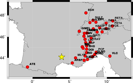
The focal mechanism was determined using broadband seismic waveforms. The location of the event and the and stations used for the waveform inversion are shown in the next figure.
|
|
|
|
The program wvfgrd96 was used with good traces observed at short distance to determine the focal mechanism, depth and seismic moment. This technique requires a high quality signal and well determined velocity model for the Green functions. To the extent that these are the quality data, this type of mechanism should be preferred over the radiation pattern technique which requires the separate step of defining the pressure and tension quadrants and the correct strike.
The observed and predicted traces are filtered using the following gsac commands:
hp c 0.03 n 3
lp c 0.06 n 3
The results of this grid search from 0.5 to 19 km depth are as follow:
           DEPTH  STK   DIP  RAKE   MW    FIT
WVFGRD96    0.5   145    40   -95   3.16 0.3424
WVFGRD96    1.0   340    50   -85   3.20 0.3520
WVFGRD96    2.0   340    50   -75   3.28 0.3851
WVFGRD96    3.0   350    55   -70   3.34 0.3612
WVFGRD96    4.0   120    35    40   3.37 0.3240
WVFGRD96    5.0    95    35     0   3.37 0.3422
WVFGRD96    6.0    90    35   -10   3.37 0.3691
WVFGRD96    7.0    90    40   -10   3.37 0.3917
WVFGRD96    8.0    95    30     5   3.43 0.4061
WVFGRD96    9.0    20    70    55   3.46 0.4245
WVFGRD96   10.0    25    65    55   3.48 0.4410
WVFGRD96   11.0    30    60    60   3.50 0.4542
WVFGRD96   12.0    35    55    65   3.53 0.4619
WVFGRD96   13.0    35    55    65   3.53 0.4659
WVFGRD96   14.0   130    45    70   3.52 0.4731
WVFGRD96   15.0   130    50    65   3.52 0.4781
WVFGRD96   16.0   125    50    60   3.53 0.4793
WVFGRD96   17.0   125    50    60   3.53 0.4780
WVFGRD96   18.0   125    50    55   3.52 0.4738
WVFGRD96   19.0   120    55    50   3.54 0.4685
WVFGRD96   20.0   120    55    50   3.54 0.4616
WVFGRD96   21.0   120    55    50   3.54 0.4542
WVFGRD96   22.0   120    55    50   3.54 0.4453
WVFGRD96   23.0   120    55    50   3.54 0.4356
WVFGRD96   24.0   120    60    45   3.56 0.4268
WVFGRD96   25.0   120    60    45   3.56 0.4174
WVFGRD96   26.0   295    60    45   3.56 0.4087
WVFGRD96   27.0   295    60    45   3.56 0.3998
WVFGRD96   28.0   295    60    40   3.57 0.3909
WVFGRD96   29.0   295    60    40   3.57 0.3821
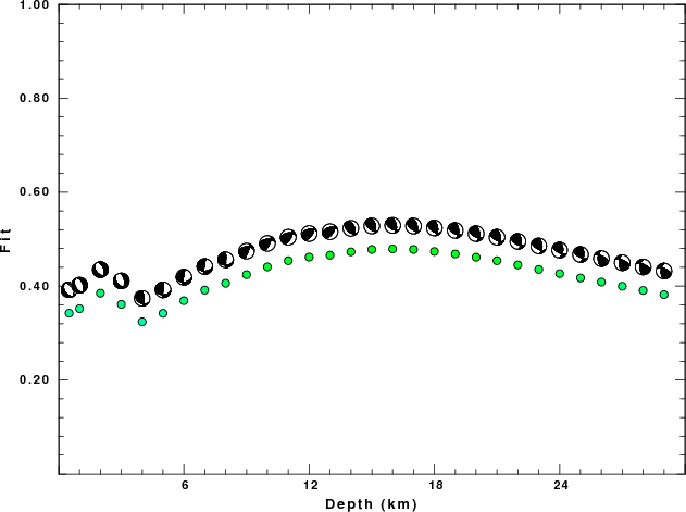
The best solution is
WVFGRD96 16.0 125 50 60 3.53 0.4793
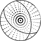
The mechanism correspond to the best fit is
|
|
|
The best fit as a function of depth is given in the following figure:
|
|
|
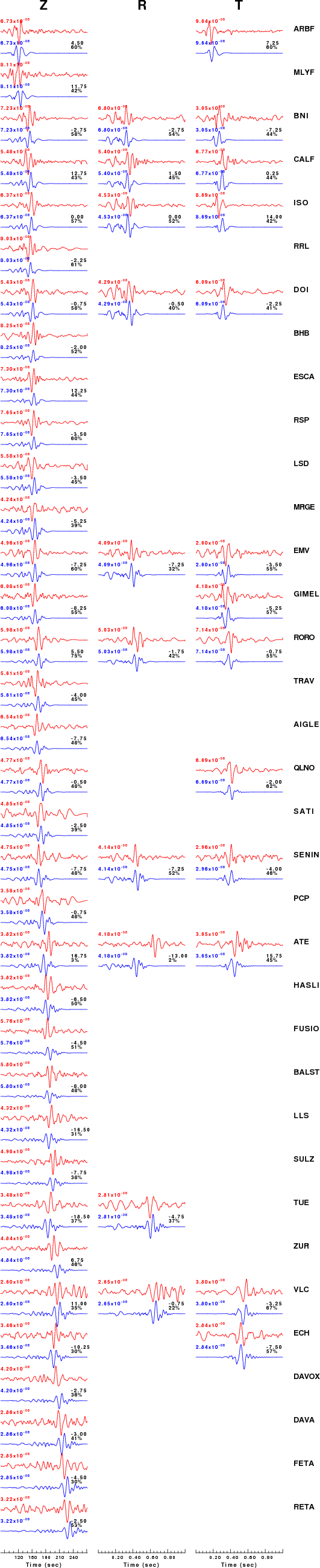
The comparison of the observed and predicted waveforms is given in the next figure. The red traces are the observed and the blue are the predicted. Each observed-predicted component is plotted to the same scale and peak amplitudes are indicated by the numbers to the left of each trace. A pair of numbers is given in black at the right of each predicted traces. The upper number it the time shift required for maximum correlation between the observed and predicted traces. This time shift is required because the synthetics are not computed at exactly the same distance as the observed and because the velocity model used in the predictions may not be perfect. A positive time shift indicates that the prediction is too fast and should be delayed to match the observed trace (shift to the right in this figure). A negative value indicates that the prediction is too slow. The lower number gives the percentage of variance reduction to characterize the individual goodness of fit (100% indicates a perfect fit).
The bandpass filter used in the processing and for the display was
hp c 0.03 n 3
lp c 0.06 n 3
|
|
|
|
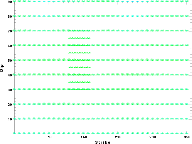
| Focal mechanism sensitivity at the preferred depth. The red color indicates a very good fit to thewavefroms. Each solution is plotted as a vector at a given value of strike and dip with the angle of the vector representing the rake angle, measured, with respect to the upward vertical (N) in the figure. |
A check on the assumed source location is possible by looking at the time shifts between the observed and predicted traces. The time shifts for waveform matching arise for several reasons:
Time_shift = A + B cos Azimuth + C Sin Azimuth
The time shifts for this inversion lead to the next figure:
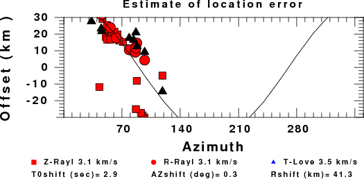
The derived shift in origin time and epicentral coordinates are given at the bottom of the figure.
Should the national backbone of the USGS Advanced National Seismic System (ANSS) be implemented with an interstation separation of 300 km, it is very likely that an earthquake such as this would have been recorded at distances on the order of 100-200 km. This means that the closest station would have information on source depth and mechanism that was lacking here.
Dr. Harley Benz, USGS, provided the USGS USNSN digital data. The digital data used in this study were provided by Natural Resources Canada through their AUTODRM site http://www.seismo.nrcan.gc.ca/nwfa/autodrm/autodrm_req_e.php, and IRIS using their BUD interface.
Thanks also to the many seismic network operators whose dedication make this effort possible: University of Alaska, University of Washington, Oregon State University, University of Utah, Montana Bureas of Mines, UC Berkely, Caltech, UC San Diego, Saint L ouis University, Universityof Memphis, Lamont Doehrty Earth Observatory, Boston College, the Iris stations and the Transportable Array of EarthScope.
The WUS used for the waveform synthetic seismograms and for the surface wave eigenfunctions and dispersion is as follows:
MODEL.01
Model after     8 iterations
ISOTROPIC
KGS
FLAT EARTH
1-D
CONSTANT VELOCITY
LINE08
LINE09
LINE10
LINE11
      H(KM)   VP(KM/S)   VS(KM/S) RHO(GM/CC)         QP         QS       ETAP       ETAS      FREFP      FREFS
     1.9000     3.4065     2.0089     2.2150  0.302E-02  0.679E-02   0.00       0.00       1.00       1.00
     6.1000     5.5445     3.2953     2.6089  0.349E-02  0.784E-02   0.00       0.00       1.00       1.00
    13.0000     6.2708     3.7396     2.7812  0.212E-02  0.476E-02   0.00       0.00       1.00       1.00
    19.0000     6.4075     3.7680     2.8223  0.111E-02  0.249E-02   0.00       0.00       1.00       1.00
     0.0000     7.9000     4.6200     3.2760  0.164E-10  0.370E-10   0.00       0.00       1.00       1.00
Here we tabulate the reasons for not using certain digital data sets
The following stations did not have a valid response files:
DATE=Thu Aug 4 07:39:27 CDT 2011