Location
IGN Location
The following location was used for the source inversion.
2010/04/22 01:24:00 35.2635 -6.2918 120.0 4.70 Moroc
SLU Location
The program
elocate
was used with the same WUS model used for the source inversion to determine the source parameters. In addition the location provided data to compare the observed first motions to the nodal planes derived from the waveform inversion. The output of this location is given in the file elocate.txt.
Focal Mechanism
 SLU Moment Tensor Solution
 ENS  2010/04/22 01:24:00:0  35.26   -6.29 120.0 4.7 Moroc

 Stations used:
   IB.NKM IG.CEUT XB.PM01 XB.PM03 XB.PM04 XB.PM05 XB.PM06
   XB.PM07 XB.PM08 XB.PM12 XB.PM13 XB.PS01 XB.PS02 XB.PS03
   XB.PS42

 Filtering commands used:
   hp c 0.02 n 3
   lp c 0.06 n 3

 Best Fitting Double Couple
  Mo = 3.67e+22 dyne-cm
  Mw = 4.31
  Z  = 70 km
  Plane   Strike  Dip  Rake
   NP1      285    57   123
   NP2       55    45    50
  Principal Axes:
   Axis    Value   Plunge  Azimuth
    T   3.67e+22     62     249
    N   0.00e+00     27      86
    P  -3.67e+22      7     352

 Moment Tensor: (dyne-cm)
    Component   Value
       Mxx    -3.46e+22
       Mxy     7.51e+21
       Mxz    -9.58e+21
       Myy     6.43e+21
       Myz    -1.37e+22
       Mzz     2.81e+22


                     --- P --------
                 -------   ------------
              ----------------------------
             ------------------------------
           ----------------------------------
          -----------------------------------#
         -----###############----------------##
        --#########################----------###
        ##############################-------###
       ##################################---#####
       ####################################-#####
       #############   ###################---####
       ############# T ##################------##
        ############   #################--------
        ##############################----------
         ###########################-----------
          #######################-------------
           ##################----------------
             ----######--------------------
              ----------------------------
                 ----------------------
                     --------------


 Global CMT Convention Moment Tensor:
      R          T          P
  2.81e+22  -9.58e+21   1.37e+22
 -9.58e+21  -3.46e+22  -7.51e+21
  1.37e+22  -7.51e+21   6.43e+21


Details of the solution is found at

http://www.eas.slu.edu/eqc/eqc_mt/MECH.NA/20100422012400/index.html
|
Preferred Solution
The preferred solution from an analysis of the surface-wave spectral amplitude radiation pattern, waveform inversion and first motion observations is
      STK = 55
      DIP = 45
     RAKE = 50
       MW = 4.31
       HS = 70.0
The waveform inversion is preferred.
Moment Tensor Comparison
The following compares this source inversion to others
| SLU |
SLUFM |
 SLU Moment Tensor Solution
 ENS  2010/04/22 01:24:00:0  35.26   -6.29 120.0 4.7 Moroc

 Stations used:
   IB.NKM IG.CEUT XB.PM01 XB.PM03 XB.PM04 XB.PM05 XB.PM06
   XB.PM07 XB.PM08 XB.PM12 XB.PM13 XB.PS01 XB.PS02 XB.PS03
   XB.PS42

 Filtering commands used:
   hp c 0.02 n 3
   lp c 0.06 n 3

 Best Fitting Double Couple
  Mo = 3.67e+22 dyne-cm
  Mw = 4.31
  Z  = 70 km
  Plane   Strike  Dip  Rake
   NP1      285    57   123
   NP2       55    45    50
  Principal Axes:
   Axis    Value   Plunge  Azimuth
    T   3.67e+22     62     249
    N   0.00e+00     27      86
    P  -3.67e+22      7     352

 Moment Tensor: (dyne-cm)
    Component   Value
       Mxx    -3.46e+22
       Mxy     7.51e+21
       Mxz    -9.58e+21
       Myy     6.43e+21
       Myz    -1.37e+22
       Mzz     2.81e+22


                     --- P --------
                 -------   ------------
              ----------------------------
             ------------------------------
           ----------------------------------
          -----------------------------------#
         -----###############----------------##
        --#########################----------###
        ##############################-------###
       ##################################---#####
       ####################################-#####
       #############   ###################---####
       ############# T ##################------##
        ############   #################--------
        ##############################----------
         ###########################-----------
          #######################-------------
           ##################----------------
             ----######--------------------
              ----------------------------
                 ----------------------
                     --------------


 Global CMT Convention Moment Tensor:
      R          T          P
  2.81e+22  -9.58e+21   1.37e+22
 -9.58e+21  -3.46e+22  -7.51e+21
  1.37e+22  -7.51e+21   6.43e+21


Details of the solution is found at

http://www.eas.slu.edu/eqc/eqc_mt/MECH.NA/20100422012400/index.html
|
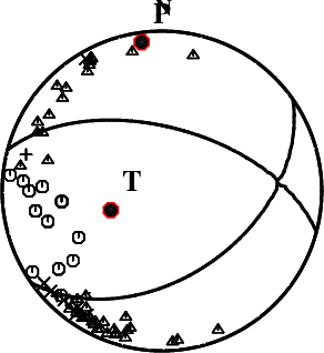
First motions and takeoff angles from an elocate run.
|
Waveform Inversion
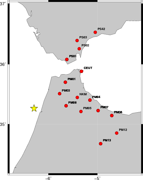
The focal mechanism was determined using broadband seismic waveforms. The location of the event and the
and stations used for the waveform inversion are shown in the next figure.
|
|
Location of broadband stations used for waveform inversion
|
The program wvfgrd96 was used with good traces observed at short distance to determine the focal mechanism, depth and seismic moment. This technique requires a high quality signal and well determined velocity model for the Green functions. To the extent that these are the quality data, this type of mechanism should be preferred over the radiation pattern technique which requires the separate step of defining the pressure and tension quadrants and the correct strike.
The observed and predicted traces are filtered using the following gsac commands:
hp c 0.02 n 3
lp c 0.06 n 3
The results of this grid search from 0.5 to 19 km depth are as follow:
           DEPTH  STK   DIP  RAKE   MW    FIT
WVFGRD96    0.5   170    50   -70   3.44 0.1403
WVFGRD96    1.0   165    50   -75   3.49 0.1451
WVFGRD96    2.0   170    50   -70   3.59 0.1781
WVFGRD96    3.0   175    55   -65   3.66 0.1785
WVFGRD96    4.0    20    40   -20   3.69 0.1749
WVFGRD96    5.0    25    45    -5   3.70 0.1906
WVFGRD96    6.0    30    45     5   3.73 0.2094
WVFGRD96    7.0    30    50    10   3.74 0.2291
WVFGRD96    8.0    30    45     5   3.80 0.2457
WVFGRD96    9.0    30    45    10   3.81 0.2631
WVFGRD96   10.0    30    45    10   3.83 0.2802
WVFGRD96   11.0    30    50    15   3.84 0.2958
WVFGRD96   12.0    30    50    10   3.85 0.3100
WVFGRD96   13.0    30    55    15   3.86 0.3224
WVFGRD96   14.0    30    55    15   3.87 0.3335
WVFGRD96   15.0    30    55    10   3.88 0.3434
WVFGRD96   16.0    30    55    10   3.89 0.3520
WVFGRD96   17.0    30    60    15   3.90 0.3594
WVFGRD96   18.0    30    60    15   3.91 0.3661
WVFGRD96   19.0    30    60    15   3.92 0.3718
WVFGRD96   20.0    30    60    15   3.92 0.3768
WVFGRD96   21.0    30    60    15   3.94 0.3806
WVFGRD96   22.0    30    60    15   3.94 0.3841
WVFGRD96   23.0    30    60    15   3.95 0.3869
WVFGRD96   24.0    30    60    15   3.96 0.3894
WVFGRD96   25.0    30    60    15   3.96 0.3912
WVFGRD96   26.0    35    60    20   3.97 0.3927
WVFGRD96   27.0    35    60    20   3.98 0.3944
WVFGRD96   28.0    35    60    20   3.99 0.3958
WVFGRD96   29.0    35    60    20   3.99 0.3968
WVFGRD96   30.0    35    60    20   4.00 0.3975
WVFGRD96   31.0    35    60    20   4.01 0.3981
WVFGRD96   32.0    35    60    20   4.01 0.3984
WVFGRD96   33.0    35    60    20   4.02 0.3984
WVFGRD96   34.0    35    60    20   4.03 0.3984
WVFGRD96   35.0    35    60    20   4.03 0.3984
WVFGRD96   36.0    35    60    20   4.04 0.3981
WVFGRD96   37.0    35    60    20   4.05 0.3979
WVFGRD96   38.0    30    65    20   4.06 0.3984
WVFGRD96   39.0    30    65    20   4.07 0.3989
WVFGRD96   40.0    40    50    25   4.16 0.3940
WVFGRD96   41.0    35    55    25   4.16 0.3962
WVFGRD96   42.0    35    55    25   4.16 0.3986
WVFGRD96   43.0    35    55    25   4.17 0.4009
WVFGRD96   44.0    35    60    30   4.18 0.4033
WVFGRD96   45.0    35    60    30   4.18 0.4054
WVFGRD96   46.0    35    60    30   4.19 0.4071
WVFGRD96   47.0    35    60    30   4.20 0.4091
WVFGRD96   48.0    35    60    30   4.20 0.4109
WVFGRD96   49.0    35    60    30   4.21 0.4122
WVFGRD96   50.0    35    60    30   4.21 0.4135
WVFGRD96   51.0    40    55    30   4.22 0.4151
WVFGRD96   52.0    40    55    35   4.23 0.4166
WVFGRD96   53.0    40    55    35   4.23 0.4182
WVFGRD96   54.0    40    55    35   4.23 0.4195
WVFGRD96   55.0    40    55    35   4.24 0.4208
WVFGRD96   56.0    40    55    35   4.24 0.4218
WVFGRD96   57.0    45    50    40   4.25 0.4234
WVFGRD96   58.0    45    50    40   4.26 0.4253
WVFGRD96   59.0    45    50    40   4.26 0.4266
WVFGRD96   60.0    45    50    40   4.27 0.4278
WVFGRD96   61.0    45    50    40   4.27 0.4288
WVFGRD96   62.0    50    45    40   4.28 0.4294
WVFGRD96   63.0    50    45    40   4.28 0.4306
WVFGRD96   64.0    50    45    40   4.28 0.4312
WVFGRD96   65.0    50    45    45   4.29 0.4317
WVFGRD96   66.0    55    45    50   4.30 0.4323
WVFGRD96   67.0    55    45    50   4.30 0.4331
WVFGRD96   68.0    55    45    50   4.31 0.4335
WVFGRD96   69.0    55    45    50   4.31 0.4337
WVFGRD96   70.0    55    45    50   4.31 0.4338
WVFGRD96   71.0    55    45    50   4.31 0.4336
WVFGRD96   72.0    55    45    50   4.32 0.4331
WVFGRD96   73.0    55    45    55   4.32 0.4325
WVFGRD96   74.0    55    45    55   4.33 0.4322
WVFGRD96   75.0    55    45    55   4.33 0.4314
WVFGRD96   76.0    55    45    55   4.33 0.4307
WVFGRD96   77.0    60    45    60   4.34 0.4299
WVFGRD96   78.0    60    45    60   4.34 0.4291
WVFGRD96   79.0    60    45    60   4.34 0.4281
WVFGRD96   80.0    60    45    60   4.34 0.4272
WVFGRD96   81.0    60    45    60   4.34 0.4257
WVFGRD96   82.0    60    45    60   4.35 0.4247
WVFGRD96   83.0    60    45    65   4.35 0.4233
WVFGRD96   84.0    60    45    65   4.36 0.4219
WVFGRD96   85.0    60    45    65   4.36 0.4205
WVFGRD96   86.0    60    45    65   4.36 0.4188
WVFGRD96   87.0    60    45    65   4.36 0.4172
WVFGRD96   88.0    65    45    70   4.37 0.4160
WVFGRD96   89.0    65    45    70   4.37 0.4146
WVFGRD96   90.0    65    45    70   4.37 0.4133
WVFGRD96   91.0    65    45    70   4.37 0.4117
WVFGRD96   92.0    65    45    70   4.37 0.4103
WVFGRD96   93.0    65    45    70   4.37 0.4084
WVFGRD96   94.0    65    45    70   4.37 0.4069
WVFGRD96   95.0    65    45    70   4.37 0.4051
WVFGRD96   96.0    65    45    70   4.38 0.4030
WVFGRD96   97.0    65    45    75   4.38 0.4014
WVFGRD96   98.0    65    45    75   4.38 0.3993
WVFGRD96   99.0    65    45    75   4.38 0.3976
WVFGRD96  100.0    70    45    80   4.39 0.3956
WVFGRD96  101.0    70    45    80   4.39 0.3939
WVFGRD96  102.0    70    45    80   4.39 0.3917
WVFGRD96  103.0    70    45    80   4.39 0.3900
WVFGRD96  104.0    70    45    80   4.39 0.3881
WVFGRD96  105.0    70    45    80   4.39 0.3859
WVFGRD96  106.0   260    45    95   4.40 0.3830
WVFGRD96  107.0   260    45    95   4.40 0.3810
WVFGRD96  108.0    70    45    80   4.40 0.3794
WVFGRD96  109.0    70    45    80   4.40 0.3776
WVFGRD96  110.0    70    45    80   4.40 0.3751
WVFGRD96  111.0    70    45    80   4.40 0.3728
WVFGRD96  112.0   260    40    90   4.41 0.3704
WVFGRD96  113.0   260    40    90   4.41 0.3689
WVFGRD96  114.0   260    40    90   4.41 0.3666
WVFGRD96  115.0    80    50    90   4.41 0.3650
WVFGRD96  116.0   260    40    90   4.41 0.3629
WVFGRD96  117.0    80    50    90   4.41 0.3606
WVFGRD96  118.0    80    50    90   4.41 0.3591
WVFGRD96  119.0   255    40    85   4.42 0.3571
WVFGRD96  120.0   255    40    85   4.42 0.3550
WVFGRD96  121.0   255    40    85   4.42 0.3532
WVFGRD96  122.0   255    40    85   4.42 0.3510
WVFGRD96  123.0   250    40    80   4.42 0.3491
WVFGRD96  124.0   250    40    80   4.42 0.3471
WVFGRD96  125.0   245    40    75   4.43 0.3449
WVFGRD96  126.0   245    40    75   4.43 0.3432
WVFGRD96  127.0   245    40    75   4.43 0.3410
WVFGRD96  128.0   240    40    70   4.44 0.3390
WVFGRD96  129.0   240    40    70   4.44 0.3374
WVFGRD96  130.0   240    40    70   4.44 0.3353
WVFGRD96  131.0   240    40    70   4.44 0.3334
WVFGRD96  132.0   235    40    65   4.45 0.3312
WVFGRD96  133.0   235    40    65   4.45 0.3299
WVFGRD96  134.0   235    40    65   4.45 0.3281
WVFGRD96  135.0   235    40    65   4.45 0.3260
WVFGRD96  136.0   235    40    60   4.46 0.3250
WVFGRD96  137.0   235    40    60   4.46 0.3230
WVFGRD96  138.0   235    40    60   4.46 0.3216
WVFGRD96  139.0   235    40    60   4.46 0.3204
The best solution is
WVFGRD96 70.0 55 45 50 4.31 0.4338
The mechanism corresponding to the best fit is
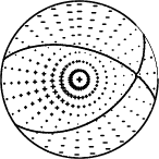
|
|
Figure 1. Waveform inversion focal mechanism
|
The best fit as a function of depth is given in the following figure:
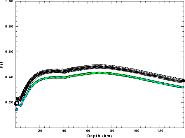
|
|
Figure 2. Depth sensitivity for waveform mechanism
|
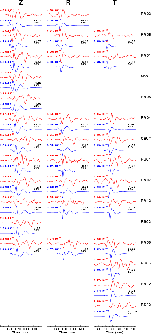
The comparison of the observed and predicted waveforms is given in the next figure. The red traces are the observed and the blue are the predicted.
Each observed-predicted component is plotted to the same scale and peak amplitudes are indicated by the numbers to the left of each trace. A pair of numbers is given in black at the right of each predicted traces. The upper number it the time shift required for maximum correlation between the observed and predicted traces. This time shift is required because the synthetics are not computed at exactly the same distance as the observed and because the velocity model used in the predictions may not be perfect.
A positive time shift indicates that the prediction is too fast and should be delayed to match the observed trace (shift to the right in this figure). A negative value indicates that the prediction is too slow. The lower number gives the percentage of variance reduction to characterize the individual goodness of fit (100% indicates a perfect fit).
The bandpass filter used in the processing and for the display was
hp c 0.02 n 3
lp c 0.06 n 3
|
|
Figure 3. Waveform comparison for selected depth
|
|
|
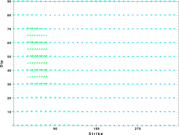
Focal mechanism sensitivity at the preferred depth. The red color indicates a very good fit to thewavefroms.
Each solution is plotted as a vector at a given value of strike and dip with the angle of the vector representing the rake angle, measured, with respect to the upward vertical (N) in the figure.
|
A check on the assumed source location is possible by looking at the time shifts between the observed and predicted traces. The time shifts for waveform matching arise for several reasons:
- The origin time and epicentral distance are incorrect
- The velocity model used for the inversion is incorrect
- The velocity model used to define the P-arrival time is not the
same as the velocity model used for the waveform inversion
(assuming that the initial trace alignment is based on the
P arrival time)
Assuming only a mislocation, the time shifts are fit to a functional form:
Time_shift = A + B cos Azimuth + C Sin Azimuth
The time shifts for this inversion lead to the next figure:
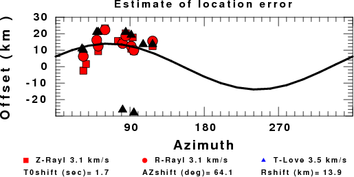
The derived shift in origin time and epicentral coordinates are given at the bottom of the figure.
Discussion
Acknowledgements
Velocity Model
The WUS used for the waveform synthetic seismograms and for the surface wave eigenfunctions and dispersion is as follows:
MODEL.01
Model after     8 iterations
ISOTROPIC
KGS
FLAT EARTH
1-D
CONSTANT VELOCITY
LINE08
LINE09
LINE10
LINE11
      H(KM)   VP(KM/S)   VS(KM/S) RHO(GM/CC)         QP         QS       ETAP       ETAS      FREFP      FREFS
     1.9000     3.4065     2.0089     2.2150  0.302E-02  0.679E-02   0.00       0.00       1.00       1.00
     6.1000     5.5445     3.2953     2.6089  0.349E-02  0.784E-02   0.00       0.00       1.00       1.00
    13.0000     6.2708     3.7396     2.7812  0.212E-02  0.476E-02   0.00       0.00       1.00       1.00
    19.0000     6.4075     3.7680     2.8223  0.111E-02  0.249E-02   0.00       0.00       1.00       1.00
     0.0000     7.9000     4.6200     3.2760  0.164E-10  0.370E-10   0.00       0.00       1.00       1.00
Quality Control
Here we tabulate the reasons for not using certain digital data sets
The following stations did not have a valid response files:
Last Changed Wed May 23 10:01:11 CEST 2012