2008/12/23 15:24:23 44.6390 10.3800 30.0 5.30
USGS Felt map for this earthquake
 USGS/SLU Moment Tensor Solution
 2008/12/23 15:24:23  44.6390  10.3800  30.0  5.30

 Best Fitting Double Couple
    Mo = 7.59e+23 dyne-cm
    Mw = 5.22
    Z  = 31 km
     Plane   Strike  Dip  Rake
      NP1       90    50    65
      NP2      306    46   117
 Principal Axes:
   Axis    Value   Plunge  Azimuth
     T   7.59e+23     71     293
     N   0.00e+00     19     107
     P  -7.59e+23      2     197


 Moment Tensor: (dyne-cm)
    Component  Value
       Mxx    -6.77e+23
       Mxy    -2.46e+23
       Mxz     1.19e+23
       Myy    -2.15e+16
       Myz    -2.06e+23
       Mzz     6.77e+23


                     --------------
                 ----------------------
              ----------------------------
             ----#####---------------------
           ##################----------------
          #######################-------------
         ##########################------------
        #############################-----------
        #############   ###############---------
       ############## T #################--------
       ##############   ##################-------
       -###################################-----#
       --###################################---##
        ---#################################-###
        ------############################---###
         ---------####################-------##
          -----------------------------------#
           ----------------------------------
             ------------------------------
              ----------------------------
                 ---   ----------------
                     P ------------


 Harvard Convention
 Moment Tensor:
      R          T          F
  6.77e+23   1.19e+23   2.06e+23
  1.19e+23  -6.77e+23   2.46e+23
  2.06e+23   2.46e+23  -2.15e+16


Details of the solution is found at

http://www.eas.slu.edu/Earthquake_Center/MECH.NA/20081223152423/index.html
|
      STK = 90
      DIP = 50
     RAKE = 65
       MW = 5.22
       HS = 31.0
The waveform inversion is preferred.
The following compares this source inversion to others
 USGS/SLU Moment Tensor Solution
 2008/12/23 15:24:23  44.6390  10.3800  30.0  5.30

 Best Fitting Double Couple
    Mo = 7.59e+23 dyne-cm
    Mw = 5.22
    Z  = 31 km
     Plane   Strike  Dip  Rake
      NP1       90    50    65
      NP2      306    46   117
 Principal Axes:
   Axis    Value   Plunge  Azimuth
     T   7.59e+23     71     293
     N   0.00e+00     19     107
     P  -7.59e+23      2     197


 Moment Tensor: (dyne-cm)
    Component  Value
       Mxx    -6.77e+23
       Mxy    -2.46e+23
       Mxz     1.19e+23
       Myy    -2.15e+16
       Myz    -2.06e+23
       Mzz     6.77e+23


                     --------------
                 ----------------------
              ----------------------------
             ----#####---------------------
           ##################----------------
          #######################-------------
         ##########################------------
        #############################-----------
        #############   ###############---------
       ############## T #################--------
       ##############   ##################-------
       -###################################-----#
       --###################################---##
        ---#################################-###
        ------############################---###
         ---------####################-------##
          -----------------------------------#
           ----------------------------------
             ------------------------------
              ----------------------------
                 ---   ----------------
                     P ------------


 Harvard Convention
 Moment Tensor:
      R          T          F
  6.77e+23   1.19e+23   2.06e+23
  1.19e+23  -6.77e+23   2.46e+23
  2.06e+23   2.46e+23  -2.15e+16


Details of the solution is found at

http://www.eas.slu.edu/Earthquake_Center/MECH.NA/20081223152423/index.html
|
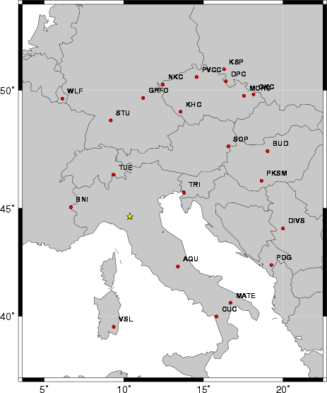
The focal mechanism was determined using broadband seismic waveforms. The location of the event and the and stations used for the waveform inversion are shown in the next figure.
|
|
|
|
The program wvfgrd96 was used with good traces observed at short distance to determine the focal mechanism, depth and seismic moment. This technique requires a high quality signal and well determined velocity model for the Green functions. To the extent that these are the quality data, this type of mechanism should be preferred over the radiation pattern technique which requires the separate step of defining the pressure and tension quadrants and the correct strike.
The observed and predicted traces are filtered using the following gsac commands:
hp c 0.02 n 3
lp c 0.05 n 3
The results of this grid search from 0.5 to 19 km depth are as follow:
           DEPTH  STK   DIP  RAKE   MW    FIT
WVFGRD96   20.0   100    55    75   5.15 0.3147
WVFGRD96   21.0   100    55    80   5.16 0.3240
WVFGRD96   22.0   100    55    75   5.17 0.3333
WVFGRD96   23.0   100    55    75   5.18 0.3420
WVFGRD96   24.0    95    55    75   5.18 0.3487
WVFGRD96   25.0    95    55    70   5.19 0.3540
WVFGRD96   26.0    95    55    70   5.19 0.3592
WVFGRD96   27.0    95    55    70   5.20 0.3627
WVFGRD96   28.0    95    50    70   5.20 0.3662
WVFGRD96   29.0    90    55    65   5.21 0.3678
WVFGRD96   30.0    90    55    65   5.22 0.3687
WVFGRD96   31.0    90    50    65   5.22 0.3696
WVFGRD96   32.0    90    50    60   5.23 0.3689
WVFGRD96   33.0    90    50    60   5.24 0.3681
WVFGRD96   34.0    90    50    60   5.25 0.3667
WVFGRD96   35.0    90    50    60   5.26 0.3641
WVFGRD96   36.0    90    50    60   5.27 0.3609
WVFGRD96   37.0    85    55    55   5.28 0.3573
WVFGRD96   38.0    85    55    55   5.29 0.3533
WVFGRD96   39.0    90    55    60   5.30 0.3486
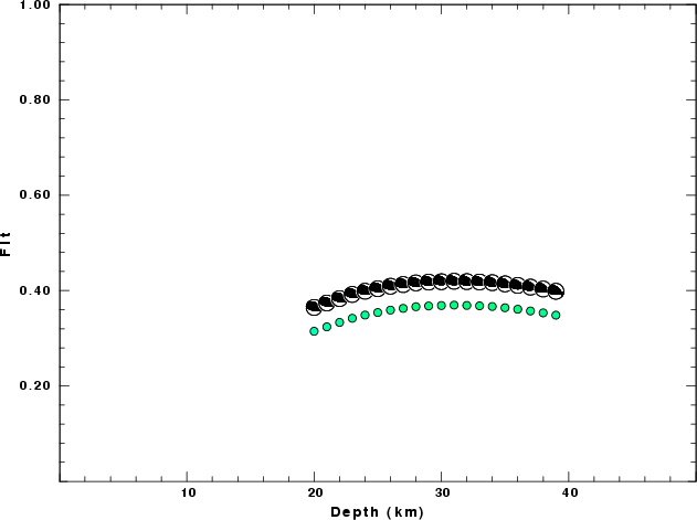
The best solution is
WVFGRD96 31.0 90 50 65 5.22 0.3696
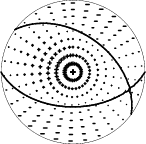
The mechanism correspond to the best fit is
|
|
|
The best fit as a function of depth is given in the following figure:
|
|
|
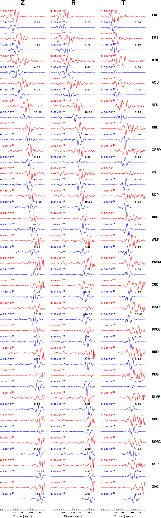
The comparison of the observed and predicted waveforms is given in the next figure. The red traces are the observed and the blue are the predicted. Each observed-predicted componnet is plotted to the same scale and peak amplitudes are indicated by the numbers to the left of each trace. The number in black at the rightr of each predicted traces it the time shift required for maximum correlation between the observed and predicted traces. This time shift is required because the synthetics are not computed at exactly the same distance as the observed and because the velocity model used in the predictions may not be perfect. A positive time shift indicates that the prediction is too fast and should be delayed to match the observed trace (shift to the right in this figure). A negative value indicates that the prediction is too slow. The bandpass filter used in the processing and for the display was
hp c 0.02 n 3
lp c 0.05 n 3
|
|
|
|
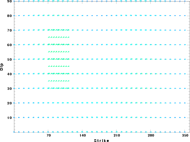
| Focal mechanism sensitivity at the preferred depth. The red color indicates a very good fit to thewavefroms. Each solution is plotted as a vector at a given value of strike and dip with the angle of the vector representing the rake angle, measured, with respect to the upward vertical (N) in the figure. |
Should the national backbone of the USGS Advanced National Seismic System (ANSS) be implemented with an interstation separation of 300 km, it is very likely that an earthquake such as this would have been recorded at distances on the order of 100-200 km. This means that the closest station would have information on source depth and mechanism that was lacking here.
Dr. Harley Benz, USGS, provided the USGS USNSN digital data. The digital data used in this study were provided by Natural Resources Canada through their AUTODRM site http://www.seismo.nrcan.gc.ca/nwfa/autodrm/autodrm_req_e.php, and IRIS using their BUD interface.
Thanks also to the many seismic network operators whose dedication make this effort possible: University of Alaska, University of Washington, Oregon State University, University of Utah, Montana Bureas of Mines, UC Berkely, Caltech, UC San Diego, Saint L ouis University, Universityof Memphis, Lamont Doehrty Earth Observatory, Boston College, the Iris stations and the Transportable Array of EarthScope.
The WUS used for the waveform synthetic seismograms and for the surface wave eigenfunctions and dispersion is as follows:
MODEL.01
Model after     8 iterations
ISOTROPIC
KGS
FLAT EARTH
1-D
CONSTANT VELOCITY
LINE08
LINE09
LINE10
LINE11
      H(KM)   VP(KM/S)   VS(KM/S) RHO(GM/CC)         QP         QS       ETAP       ETAS      FREFP      FREFS
     1.9000     3.4065     2.0089     2.2150  0.302E-02  0.679E-02   0.00       0.00       1.00       1.00
     6.1000     5.5445     3.2953     2.6089  0.349E-02  0.784E-02   0.00       0.00       1.00       1.00
    13.0000     6.2708     3.7396     2.7812  0.212E-02  0.476E-02   0.00       0.00       1.00       1.00
    19.0000     6.4075     3.7680     2.8223  0.111E-02  0.249E-02   0.00       0.00       1.00       1.00
     0.0000     7.9000     4.6200     3.2760  0.164E-10  0.370E-10   0.00       0.00       1.00       1.00
Here we tabulate the reasons for not using certain digital data sets
The following stations did not have a valid response files:
DATE=Tue Dec 23 10:57:35 MST 2008