2008/06/24 18:26:52 40.148 70.762 38.2 5.0 state
USGS Felt map for this earthquake
 USGS/SLU Moment Tensor Solution
 2008/06/24 18:26:52 40.148 70.762 38.2 5.0 state

 Best Fitting Double Couple
    Mo = 9.23e+22 dyne-cm
    Mw = 4.61
    Z  = 26 km
     Plane   Strike  Dip  Rake
      NP1      287    74   102
      NP2       70    20    55
 Principal Axes:
   Axis    Value   Plunge  Azimuth
     T   9.23e+22     60     213
     N   0.00e+00     11     103
     P  -9.23e+22     28       7


 Moment Tensor: (dyne-cm)
    Component  Value
       Mxx    -5.45e+22
       Mxy     1.75e+21
       Mxz    -7.14e+22
       Myy     5.95e+21
       Myz    -2.69e+22
       Mzz     4.86e+22


                     --------------
                 -----------   --------
              -------------- P -----------
             ---------------   ------------
           ----------------------------------
          ------------------------------------
         --------------------------------------
        ----####--------------------------------
        ###################---------------------
       ##########################---------------#
       ##############################-----------#
       ##################################------##
       #####################################---##
        ##############   #######################
        ############## T ####################---
         #############   ###################---
          -###############################----
           --###########################-----
             --#######################-----
              -----###############--------
                 ----------------------
                     --------------


 Harvard Convention
 Moment Tensor:
      R          T          F
  4.86e+22  -7.14e+22   2.69e+22
 -7.14e+22  -5.45e+22  -1.75e+21
  2.69e+22  -1.75e+21   5.95e+21


Details of the solution is found at

http://www.eas.slu.edu/Earthquake_Center/MECH.NA/20080624182652/index.html
|
      STK = 70
      DIP = 20
     RAKE = 55
       MW = 4.61
       HS = 26
The surface-wave is preferred. Rake is least well determined.
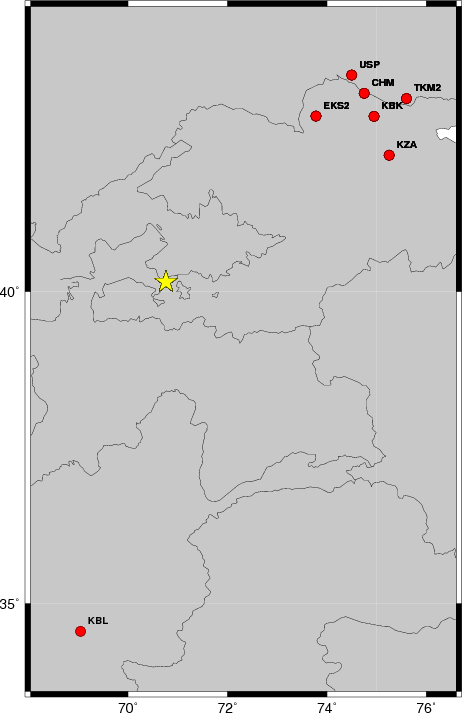
The focal mechanism was determined using broadband seismic waveforms. The location of the event and the and stations used for the waveform inversion are shown in the next figure.
|
|
|
|
The program wvfgrd96 was used with good traces observed at short distance to determine the focal mechanism, depth and seismic moment. This technique requires a high quality signal and well determined velocity model for the Green functions. To the extent that these are the quality data, this type of mechanism should be preferred over the radiation pattern technique which requires the separate step of defining the pressure and tension quadrants and the correct strike.
The observed and predicted traces are filtered using the following gsac commands:
hp c 0.02 n 3
lp c 0.05 n 3
br c 0.12 0.25 n 4 p 2
The results of this grid search from 0.5 to 19 km depth are as follow:
           DEPTH  STK   DIP  RAKE   MW    FIT
WVFGRD96    0.5   170    50   -70   4.29 0.4758
WVFGRD96    1.0   185    75   -15   4.35 0.4752
WVFGRD96    2.0   175    50   -45   4.38 0.5099
WVFGRD96    3.0   170    40   -50   4.46 0.5278
WVFGRD96    4.0   165    35   -55   4.53 0.5396
WVFGRD96    5.0   165    35   -50   4.57 0.5301
WVFGRD96    6.0   185    65     0   4.58 0.5142
WVFGRD96    7.0   185    70     5   4.61 0.5038
WVFGRD96    8.0   185    65    10   4.64 0.4874
WVFGRD96    9.0   185    70    15   4.65 0.4728
WVFGRD96   10.0    35    50    65   4.70 0.4754
WVFGRD96   11.0    35    50    65   4.70 0.5095
WVFGRD96   12.0    35    50    65   4.70 0.5435
WVFGRD96   13.0    35    45    60   4.68 0.5679
WVFGRD96   14.0    35    45    60   4.68 0.5855
WVFGRD96   15.0    35    45    60   4.68 0.6088
WVFGRD96   16.0   105    30    75   4.57 0.6258
WVFGRD96   17.0   105    25    85   4.57 0.6496
WVFGRD96   18.0   100    25    80   4.57 0.6722
WVFGRD96   19.0   100    25    80   4.57 0.6826
WVFGRD96   20.0    90    25    70   4.57 0.6963
WVFGRD96   21.0    90    25    70   4.59 0.7030
WVFGRD96   22.0    85    25    65   4.59 0.7074
WVFGRD96   23.0    85    20    70   4.60 0.7141
WVFGRD96   24.0    80    20    65   4.60 0.7173
WVFGRD96   25.0    75    20    60   4.61 0.7192
WVFGRD96   26.0    70    20    55   4.61 0.7225
WVFGRD96   27.0    70    20    55   4.62 0.7195
WVFGRD96   28.0    65    20    50   4.62 0.7169
WVFGRD96   29.0    60    20    45   4.63 0.7151
The best solution is
WVFGRD96 26.0 70 20 55 4.61 0.7225
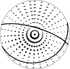
The mechanism correspond to the best fit is
|
|
|
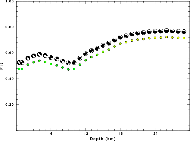
The best fit as a function of depth is given in the following figure:
|
|
|
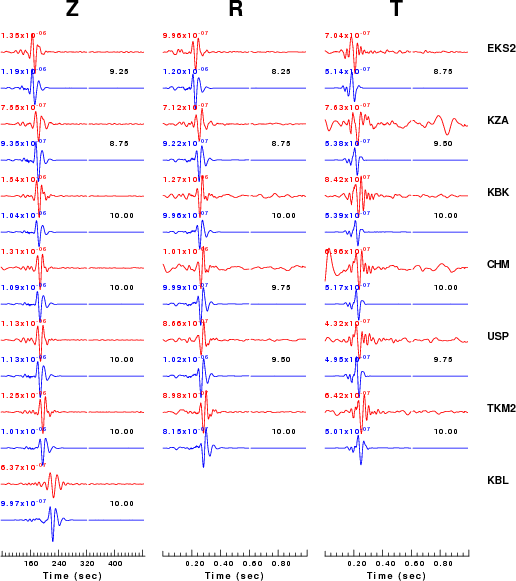
The comparison of the observed and predicted waveforms is given in the next figure. The red traces are the observed and the blue are the predicted. Each observed-predicted componnet is plotted to the same scale and peak amplitudes are indicated by the numbers to the left of each trace. The number in black at the rightr of each predicted traces it the time shift required for maximum correlation between the observed and predicted traces. This time shift is required because the synthetics are not computed at exactly the same distance as the observed and because the velocity model used in the predictions may not be perfect. A positive time shift indicates that the prediction is too fast and should be delayed to match the observed trace (shift to the right in this figure). A negative value indicates that the prediction is too slow. The bandpass filter used in the processing and for the display was
hp c 0.02 n 3
lp c 0.05 n 3
br c 0.12 0.25 n 4 p 2
|
|
|
|
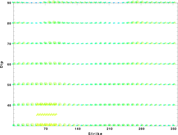
| Focal mechanism sensitivity at the preferred depth. The red color indicates a very good fit to thewavefroms. Each solution is plotted as a vector at a given value of strike and dip with the angle of the vector representing the rake angle, measured, with respect to the upward vertical (N) in the figure. |
The following figure shows the stations used in the grid search for the best focal mechanism to fit the surface-wave spectral amplitudes of the Love and Rayleigh waves.

|
|
|
The surface-wave determined focal mechanism is shown here.
 |
The P-wave first motion data for focal mechanism studies are as follow:
Sta Az(deg)    Dist(km)   First motion
EKS2       41  376 -12345
KZA        59  434 -12345
KBK        50  447 -12345
CHM        45  459 -12345
USP        41  465 -12345
TKM2       51  507 -12345
KBL       194  641 -12345
Surface wave analysis was performed using codes from Computer Programs in Seismology, specifically the multiple filter analysis program do_mft and the surface-wave radiation pattern search program srfgrd96.
Digital data were collected, instrument response removed and traces converted
to Z, R an T components. Multiple filter analysis was applied to the Z and T traces to obtain the Rayleigh- and Love-wave spectral amplitudes, respectively.
These were input to the search program which examined all depths between 1 and 25 km
and all possible mechanisms.

|
|
|

|
| Pressure-tension axis trends. Since the surface-wave spectra search does not distinguish between P and T axes and since there is a 180 ambiguity in strike, all possible P and T axes are plotted. First motion data and waveforms will be used to select the preferred mechanism. The purpose of this plot is to provide an idea of the possible range of solutions. The P and T-axes for all mechanisms with goodness of fit greater than 0.9 FITMAX (above) are plotted here. |

|
| Focal mechanism sensitivity at the preferred depth. The red color indicates a very good fit to the Love and Rayleigh wave radiation patterns. Each solution is plotted as a vector at a given value of strike and dip with the angle of the vector representing the rake angle, measured, with respect to the upward vertical (N) in the figure. Because of the symmetry of the spectral amplitude rediation patterns, only strikes from 0-180 degrees are sampled. |
The distribution of broadband stations with azimuth and distance is
Sta Az(deg) Dist(km)
Since the analysis of the surface-wave radiation patterns uses only spectral amplitudes and because the surfave-wave radiation patterns have a 180 degree symmetry, each surface-wave solution consists of four possible focal mechanisms corresponding to the interchange of the P- and T-axes and a roation of the mechanism by 180 degrees. To select one mechanism, P-wave first motion can be used. This was not possible in this case because all the P-wave first motions were emergent ( a feature of the P-wave wave takeoff angle, the station location and the mechanism). The other way to select among the mechanisms is to compute forward synthetics and compare the observed and predicted waveforms.
The fits to the waveforms with the given mechanism are show below:

|
This figure shows the fit to the three components of motion (Z - vertical, R-radial and T - transverse). For each station and component, the observed traces is shown in red and the model predicted trace in blue. The traces represent filtered ground velocity in units of meters/sec (the peak value is printed adjacent to each trace; each pair of traces to plotted to the same scale to emphasize the difference in levels). Both synthetic and observed traces have been filtered using the SAC commands:

|

|
Should the national backbone of the USGS Advanced National Seismic System (ANSS) be implemented with an interstation separation of 300 km, it is very likely that an earthquake such as this would have been recorded at distances on the order of 100-200 km. This means that the closest station would have information on source depth and mechanism that was lacking here.
Dr. Harley Benz, USGS, provided the USGS USNSN digital data. The digital data used in this study were provided by Natural Resources Canada through their AUTODRM site http://www.seismo.nrcan.gc.ca/nwfa/autodrm/autodrm_req_e.php, and IRIS using their BUD interface
The WUS.REG used for the waveform synthetic seismograms and for the surface wave eigenfunctions and dispersion is as follows:
MODEL.01
Model after     8 iterations
ISOTROPIC
KGS
FLAT EARTH
1-D
CONSTANT VELOCITY
LINE08
LINE09
LINE10
LINE11
      H(KM)   VP(KM/S)   VS(KM/S) RHO(GM/CC)         QP         QS       ETAP       ETAS      FREFP      FREFS
     1.9000     3.4065     2.0089     2.2150  0.302E-02  0.679E-02   0.00       0.00       1.00       1.00
     6.1000     5.5445     3.2953     2.6089  0.349E-02  0.784E-02   0.00       0.00       1.00       1.00
    13.0000     6.2708     3.7396     2.7812  0.212E-02  0.476E-02   0.00       0.00       1.00       1.00
    19.0000     6.4075     3.7680     2.8223  0.111E-02  0.249E-02   0.00       0.00       1.00       1.00
     0.0000     7.9000     4.6200     3.2760  0.164E-10  0.370E-10   0.00       0.00       1.00       1.00
Here we tabulate the reasons for not using certain digital data sets
The following stations did not have a valid response files:
DATE=Wed Jun 25 20:02:58 MDT 2008