2008/03/01 08:43:49 44.23 11.20 10.0 4.6 Italy
USGS Felt map for this earthquake
 SLU Moment Tensor Solution
 2008/03/01 08:43:49 44.23 11.20 10.0 4.6 Italy

 Best Fitting Double Couple
    Mo = 1.84e+22 dyne-cm
    Mw = 4.11
    Z  = 8 km
     Plane   Strike  Dip  Rake
      NP1      276    52   -117
      NP2      135    45   -60
 Principal Axes:
   Axis    Value   Plunge  Azimuth
     T   1.84e+22      4      24
     N   0.00e+00     21     293
     P  -1.84e+22     69     124


 Moment Tensor: (dyne-cm)
    Component  Value
       Mxx     1.45e+22
       Mxy     7.97e+21
       Mxz     4.60e+21
       Myy     1.46e+21
       Myz    -4.60e+21
       Mzz    -1.59e+22


                     ##############
                 ################## T #
              #####################   ####
             ##############################
           --################################
          --##################################
         ---#####------------------############
        -------------------------------#########
        --###------------------------------#####
       -#####--------------------------------####
       #######---------------------------------##
       ########----------------   --------------#
       #########--------------- P ---------------
        #########--------------   --------------
        ###########-----------------------------
         ###########---------------------------
          #############-----------------------
           ##############--------------------
             ################--------------
              ############################
                 ######################
                     ##############


 Harvard Convention
 Moment Tensor:
      R          T          F
 -1.59e+22   4.60e+21   4.60e+21
  4.60e+21   1.45e+22  -7.97e+21
  4.60e+21  -7.97e+21   1.46e+21


Details of the solution is found at

http://www.eas.slu.edu/Earthquake_Center/MECH.NA/20080301084349/index.html
|
      STK = 135
      DIP = 45
     RAKE = -60
       MW = 4.11
       HS = 8.0
The waveform inversion is preferred.
The following compares this source inversion to others
 SLU Moment Tensor Solution
 2008/03/01 08:43:49 44.23 11.20 10.0 4.6 Italy

 Best Fitting Double Couple
    Mo = 1.84e+22 dyne-cm
    Mw = 4.11
    Z  = 8 km
     Plane   Strike  Dip  Rake
      NP1      276    52   -117
      NP2      135    45   -60
 Principal Axes:
   Axis    Value   Plunge  Azimuth
     T   1.84e+22      4      24
     N   0.00e+00     21     293
     P  -1.84e+22     69     124


 Moment Tensor: (dyne-cm)
    Component  Value
       Mxx     1.45e+22
       Mxy     7.97e+21
       Mxz     4.60e+21
       Myy     1.46e+21
       Myz    -4.60e+21
       Mzz    -1.59e+22


                     ##############
                 ################## T #
              #####################   ####
             ##############################
           --################################
          --##################################
         ---#####------------------############
        -------------------------------#########
        --###------------------------------#####
       -#####--------------------------------####
       #######---------------------------------##
       ########----------------   --------------#
       #########--------------- P ---------------
        #########--------------   --------------
        ###########-----------------------------
         ###########---------------------------
          #############-----------------------
           ##############--------------------
             ################--------------
              ############################
                 ######################
                     ##############


 Harvard Convention
 Moment Tensor:
      R          T          F
 -1.59e+22   4.60e+21   4.60e+21
  4.60e+21   1.45e+22  -7.97e+21
  4.60e+21  -7.97e+21   1.46e+21


Details of the solution is found at

http://www.eas.slu.edu/Earthquake_Center/MECH.NA/20080301084349/index.html
|
EMSC Moment Tensors solutions

Provided by ETHZ, AUTH, IGN, INGV-MEDNET, KOERI, NOA_IG, HARVARD, USGS, CPPT

From: pondrix@bo.ingv.it
FID: AVY24
DAT: 200803011019 GMT
MW=4.23

S030108A 03/01/08 08:43:50.0  44.15   11.23  10.04.60.0NORTHERN ITALY
Nei BW: 0  0   0 SW: 8 11  30 DT=   7.7 1.6  44.50 0.09   11.36 0.08  18.8  3.1
 DUR 0.3 EX 22  1.99 0.45 -2.95 0.40  0.96 0.21  0.97 0.41  0.44 0.32  0.50 0.20
   2.37 66 299   0.80 22  92  -3.18 10 186   2.77 300 40  125  78 59   65
CENTROID, MOMENT TENSOR SOLUTION
HARVARD EVENT-FILE NAME S030108A
DATA USED: GSN
SURFACE WAVES:    8S, 11C, T= 30
CENTROID LOCATION:
ORIGIN TIME       08:43:57.7 1.6
LAT 44.50N 0.09;LON  11.36E 0.08
DEP  18.8 3.1;HALF-DURATION  0.3
MOMENT TENSOR; SCALE 10**22 D-CM
  MRR= 1.99 0.45; MTT=-2.95 0.40
  MPP= 0.96 0.21; MRT= 0.97 0.41
  MRP= 0.44 0.32; MTP= 0.50 0.20
 PRINCIPAL AXES:
 1.(T) VAL=  2.37;PLG=66;AZM=299
 2.(N)       0.80;    22;     92
 3.(P)      -3.18;    10;    186
BEST DOUBLE COUPLE:M0=2.8*10**22
 NP1:STRIKE=300;DIP=40;SLIP= 125
 NP2:STRIKE= 78;DIP=59;SLIP=  65

            -----------
        -------------------
      -----------------------
    --#############------------
   ####################---------
  ########################-------
  ##########   ############------
 ########### T ##############----#
 ###########   ###############--##
 #############################-###
 ###########################---###
  -#####################--------#
  ------##########--------------#
   -----------------------------
    ---------------------------
      -----------------------
        ------   ----------
            -- P ------
|
Per scaricare l'immagine, click con il tasto destro e scegliere salva... |
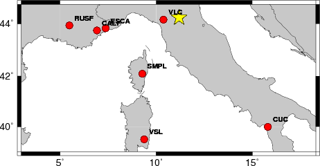
The focal mechanism was determined using broadband seismic waveforms. The location of the event and the and stations used for the waveform inversion are shown in the next figure.
|
|
|
|
The program wvfgrd96 was used with good traces observed at short distance to determine the focal mechanism, depth and seismic moment. This technique requires a high quality signal and well determined velocity model for the Green functions. To the extent that these are the quality data, this type of mechanism should be preferred over the radiation pattern technique which requires the separate step of defining the pressure and tension quadrants and the correct strike.
The observed and predicted traces are filtered using the following gsac commands:
hp c 0.02 n 3
lp c 0.05 n 3
br c 0.12 0.25 n 4 p 2
The results of this grid search from 0.5 to 19 km depth are as follow:
           DEPTH  STK   DIP  RAKE   MW    FIT
WVFGRD96    0.5   180    70   -25   3.78 0.2964
WVFGRD96    1.0    10    85     5   3.80 0.3150
WVFGRD96    2.0   175    65   -25   3.89 0.3883
WVFGRD96    3.0   170    75   -40   3.95 0.4048
WVFGRD96    4.0   335    75   -45   4.01 0.4363
WVFGRD96    5.0   335    70   -40   4.01 0.4572
WVFGRD96    6.0   330    60   -40   4.04 0.4708
WVFGRD96    7.0   330    55   -40   4.06 0.4804
WVFGRD96    8.0   325    55   -45   4.10 0.4850
WVFGRD96    9.0   330    60   -40   4.08 0.4862
WVFGRD96   10.0   330    55   -40   4.09 0.4852
WVFGRD96   11.0   335    60   -30   4.08 0.4820
WVFGRD96   12.0   335    60   -30   4.08 0.4785
WVFGRD96   13.0   335    60   -30   4.09 0.4759
WVFGRD96   14.0   335    60   -30   4.09 0.4742
WVFGRD96   15.0   335    60   -25   4.10 0.4733
WVFGRD96   16.0   335    60   -25   4.11 0.4716
WVFGRD96   17.0   335    60   -25   4.11 0.4694
WVFGRD96   18.0   335    60   -25   4.12 0.4665
WVFGRD96   19.0   335    55   -20   4.14 0.4639
WVFGRD96   20.0   335    55   -20   4.15 0.4613
WVFGRD96   21.0   335    55   -20   4.16 0.4586
WVFGRD96   22.0   335    60   -20   4.16 0.4558
WVFGRD96   23.0   335    60   -20   4.16 0.4529
WVFGRD96   24.0   335    60   -20   4.17 0.4494
WVFGRD96   25.0   335    60   -20   4.18 0.4458
WVFGRD96   26.0   335    60   -20   4.18 0.4419
WVFGRD96   27.0   335    60   -20   4.19 0.4375
WVFGRD96   28.0   335    55    -5   4.23 0.4343
WVFGRD96   29.0   335    55    -5   4.24 0.4310
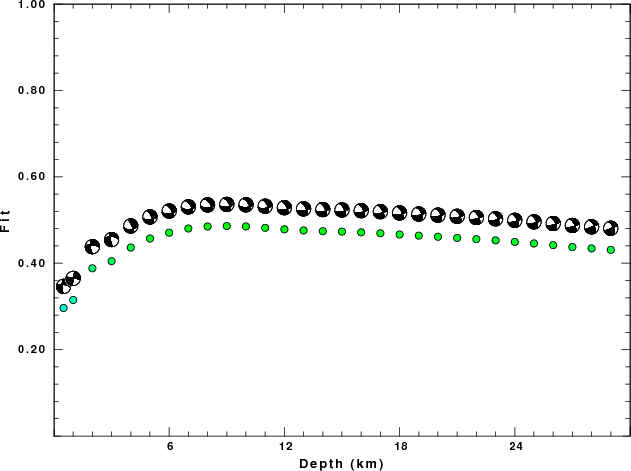
The best solution is
WVFGRD96 9.0 330 60 -40 4.08 0.4862
The mechanism correspond to the best fit is
|
|
|
The best fit as a function of depth is given in the following figure:
|
|
|
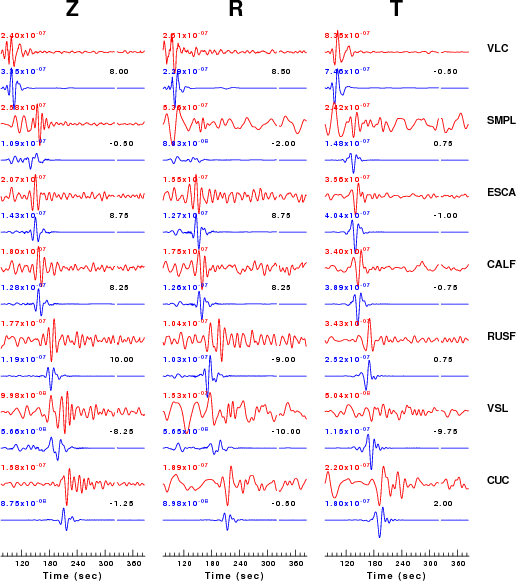
The comparison of the observed and predicted waveforms is given in the next figure. The red traces are the observed and the blue are the predicted. Each observed-predicted componnet is plotted to the same scale and peak amplitudes are indicated by the numbers to the left of each trace. The number in black at the rightr of each predicted traces it the time shift required for maximum correlation between the observed and predicted traces. This time shift is required because the synthetics are not computed at exactly the same distance as the observed and because the velocity model used in the predictions may not be perfect. A positive time shift indicates that the prediction is too fast and should be delayed to match the observed trace (shift to the right in this figure). A negative value indicates that the prediction is too slow. The bandpass filter used in the processing and for the display was
hp c 0.02 n 3
lp c 0.05 n 3
br c 0.12 0.25 n 4 p 2
|
|
|
|
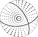
| Focal mechanism sensitivity at the preferred depth. The red color indicates a very good fit to thewavefroms. Each solution is plotted as a vector at a given value of strike and dip with the angle of the vector representing the rake angle, measured, with respect to the upward vertical (N) in the figure. |
The following figure shows the stations used in the grid search for the best focal mechanism to fit the surface-wave spectral amplitudes of the Love and Rayleigh waves.

|
|
|
The surface-wave determined focal mechanism is shown here.
 |
The P-wave first motion data for focal mechanism studies are as follow:
Sta Az(deg)    Dist(km)   First motion
VLC       263   66 -12345
SMPL      214  284 -12345
ESCA      263  310 -12345
CALF      263  347 -12345
RUSF      268  459 -12345
VSL       197  547 -12345
CUC       139  606 -12345
Surface wave analysis was performed using codes from Computer Programs in Seismology, specifically the multiple filter analysis program do_mft and the surface-wave radiation pattern search program srfgrd96.
Digital data were collected, instrument response removed and traces converted
to Z, R an T components. Multiple filter analysis was applied to the Z and T traces to obtain the Rayleigh- and Love-wave spectral amplitudes, respectively.
These were input to the search program which examined all depths between 1 and 25 km
and all possible mechanisms.

|
|
|

|
| Pressure-tension axis trends. Since the surface-wave spectra search does not distinguish between P and T axes and since there is a 180 ambiguity in strike, all possible P and T axes are plotted. First motion data and waveforms will be used to select the preferred mechanism. The purpose of this plot is to provide an idea of the possible range of solutions. The P and T-axes for all mechanisms with goodness of fit greater than 0.9 FITMAX (above) are plotted here. |

|
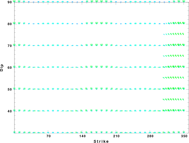
| Focal mechanism sensitivity at the preferred depth. The red color indicates a very good fit to the Love and Rayleigh wave radiation patterns. Each solution is plotted as a vector at a given value of strike and dip with the angle of the vector representing the rake angle, measured, with respect to the upward vertical (N) in the figure. Because of the symmetry of the spectral amplitude rediation patterns, only strikes from 0-180 degrees are sampled. |
The distribution of broadband stations with azimuth and distance is
Sta Az(deg) Dist(km)
Since the analysis of the surface-wave radiation patterns uses only spectral amplitudes and because the surfave-wave radiation patterns have a 180 degree symmetry, each surface-wave solution consists of four possible focal mechanisms corresponding to the interchange of the P- and T-axes and a roation of the mechanism by 180 degrees. To select one mechanism, P-wave first motion can be used. This was not possible in this case because all the P-wave first motions were emergent ( a feature of the P-wave wave takeoff angle, the station location and the mechanism). The other way to select among the mechanisms is to compute forward synthetics and compare the observed and predicted waveforms.
The fits to the waveforms with the given mechanism are show below:

|
This figure shows the fit to the three components of motion (Z - vertical, R-radial and T - transverse). For each station and component, the observed traces is shown in red and the model predicted trace in blue. The traces represent filtered ground velocity in units of meters/sec (the peak value is printed adjacent to each trace; each pair of traces to plotted to the same scale to emphasize the difference in levels). Both synthetic and observed traces have been filtered using the SAC commands:

|

|
Should the national backbone of the USGS Advanced National Seismic System (ANSS) be implemented with an interstation separation of 300 km, it is very likely that an earthquake such as this would have been recorded at distances on the order of 100-200 km. This means that the closest station would have information on source depth and mechanism that was lacking here.
Dr. Harley Benz, USGS, provided the USGS USNSN digital data. The digital data used in this study were provided by Natural Resources Canada through their AUTODRM site http://www.seismo.nrcan.gc.ca/nwfa/autodrm/autodrm_req_e.php, and IRIS using their BUD interface.
Thanks also to the many seismic network operators whose dedication make this effort possible: University of Alaska, University of Washington, Oregon State University, University of Utah, Montana Bureas of Mines, UC Berkely, Caltech, UC San Diego, Saint L ouis University, Universityof Memphis, Lamont Doehrty Earth Observatory, Boston College, the Iris stations and the Transportable Array of EarthScope.
The WUS used for the waveform synthetic seismograms and for the surface wave eigenfunctions and dispersion is as follows:
MODEL.01
Model after     8 iterations
ISOTROPIC
KGS
FLAT EARTH
1-D
CONSTANT VELOCITY
LINE08
LINE09
LINE10
LINE11
      H(KM)   VP(KM/S)   VS(KM/S) RHO(GM/CC)         QP         QS       ETAP       ETAS      FREFP      FREFS
     1.9000     3.4065     2.0089     2.2150  0.302E-02  0.679E-02   0.00       0.00       1.00       1.00
     6.1000     5.5445     3.2953     2.6089  0.349E-02  0.784E-02   0.00       0.00       1.00       1.00
    13.0000     6.2708     3.7396     2.7812  0.212E-02  0.476E-02   0.00       0.00       1.00       1.00
    19.0000     6.4075     3.7680     2.8223  0.111E-02  0.249E-02   0.00       0.00       1.00       1.00
     0.0000     7.9000     4.6200     3.2760  0.164E-10  0.370E-10   0.00       0.00       1.00       1.00
Here we tabulate the reasons for not using certain digital data sets
The following stations did not have a valid response files:
DATE=Mon Mar 3 08:30:08 CST 2008