Location

2007/08/12 07:47:05 39.3743 -2.9894 16 4.70 Spain

Focal Mechanism

USGS/SLU Moment Tensor Solution ENS 2007/08/12 07:47:05:0 39.37 -2.99 16.0 4.7 Spain Stations used: CA.CMAS ES.EADA ES.EBAD ES.EBEN ES.EBER ES.ECAL ES.EMIN ES.EMOS ES.EMUR ES.EQES ES.EQTA ES.ERTA ES.ESAC ES.ESBB ES.ETOB IB.E020 IB.E025 IB.EHUE IB.ELOJ IB.ELUQ IG.ACBG IG.ACLR IG.ANER IG.ARAC IG.ASCB IG.ESTP IG.GORA IG.HORN IG.JAND IG.ROMA IG.SELV IG.SESP IG.XIII PM.MVO PM.PESTR PM.PMRV Filtering commands used: hp c 0.02 n 3 lp c 0.06 n 3 Best Fitting Double Couple Mo = 1.11e+23 dyne-cm Mw = 4.63 Z = 11 km Plane Strike Dip Rake NP1 245 85 175 NP2 335 85 5 Principal Axes: Axis Value Plunge Azimuth T 1.11e+23 7 200 N 0.00e+00 83 20 P -1.11e+23 0 290 Moment Tensor: (dyne-cm) Component Value Mxx 8.40e+22 Mxy 7.01e+22 Mxz -1.28e+22 Myy -8.57e+22 Myz -4.56e+21 Mzz 1.68e+21 ############## ---################### -------##################### ---------##################### ------------###################### --------------###################### ---------------####################-- P ----------------##############-------- -----------------########------------- ---------------------###------------------ --------------------##-------------------- ----------------#######------------------- -------------###########------------------ --------###############----------------- -----###################---------------- -#######################-------------- ########################------------ ########################---------- ######################-------- ###### #############------ ### T #############--- ############ Global CMT Convention Moment Tensor: R T P 1.68e+21 -1.28e+22 4.56e+21 -1.28e+22 8.40e+22 -7.01e+22 4.56e+21 -7.01e+22 -8.57e+22 Details of the solution is found at http://www.eas.slu.edu/eqc/eqc_mt/MECH.NA/20070812074705/index.html

Preferred Solution

The preferred solution from an analysis of the surface-wave spectral amplitude radiation pattern, waveform inversion and first motion observations is

      STK = 335
      DIP = 85
     RAKE = 5
       MW = 4.63
       HS = 11.0

The waveform inversion is preferred.

Moment Tensor Comparison

The following compares this source inversion to others

SLU

USGS/SLU Moment Tensor Solution ENS 2007/08/12 07:47:05:0 39.37 -2.99 16.0 4.7 Spain Stations used: CA.CMAS ES.EADA ES.EBAD ES.EBEN ES.EBER ES.ECAL ES.EMIN ES.EMOS ES.EMUR ES.EQES ES.EQTA ES.ERTA ES.ESAC ES.ESBB ES.ETOB IB.E020 IB.E025 IB.EHUE IB.ELOJ IB.ELUQ IG.ACBG IG.ACLR IG.ANER IG.ARAC IG.ASCB IG.ESTP IG.GORA IG.HORN IG.JAND IG.ROMA IG.SELV IG.SESP IG.XIII PM.MVO PM.PESTR PM.PMRV Filtering commands used: hp c 0.02 n 3 lp c 0.06 n 3 Best Fitting Double Couple Mo = 1.11e+23 dyne-cm Mw = 4.63 Z = 11 km Plane Strike Dip Rake NP1 245 85 175 NP2 335 85 5 Principal Axes: Axis Value Plunge Azimuth T 1.11e+23 7 200 N 0.00e+00 83 20 P -1.11e+23 0 290 Moment Tensor: (dyne-cm) Component Value Mxx 8.40e+22 Mxy 7.01e+22 Mxz -1.28e+22 Myy -8.57e+22 Myz -4.56e+21 Mzz 1.68e+21 ############## ---################### -------##################### ---------##################### ------------###################### --------------###################### ---------------####################-- P ----------------##############-------- -----------------########------------- ---------------------###------------------ --------------------##-------------------- ----------------#######------------------- -------------###########------------------ --------###############----------------- -----###################---------------- -#######################-------------- ########################------------ ########################---------- ######################-------- ###### #############------ ### T #############--- ############ Global CMT Convention Moment Tensor: R T P 1.68e+21 -1.28e+22 4.56e+21 -1.28e+22 8.40e+22 -7.01e+22 4.56e+21 -7.01e+22 -8.57e+22 Details of the solution is found at http://www.eas.slu.edu/eqc/eqc_mt/MECH.NA/20070812074705/index.html

Waveform Inversion

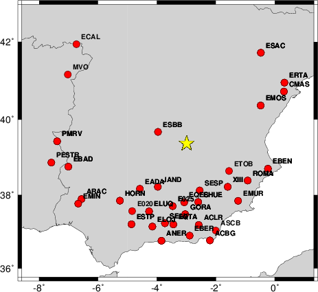
The focal mechanism was determined using broadband seismic waveforms. The location of the event and the and stations used for the waveform inversion are shown in the next figure.

Location of broadband stations used for waveform inversion

The program wvfgrd96 was used with good traces observed at short distance to determine the focal mechanism, depth and seismic moment. This technique requires a high quality signal and well determined velocity model for the Green functions. To the extent that these are the quality data, this type of mechanism should be preferred over the radiation pattern technique which requires the separate step of defining the pressure and tension quadrants and the correct strike.

The observed and predicted traces are filtered using the following gsac commands:

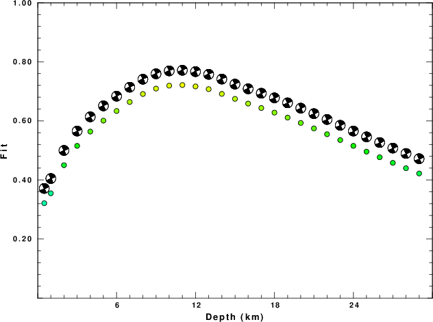
hp c 0.02 n 3
lp c 0.06 n 3

The results of this grid search from 0.5 to 19 km depth are as follow:

           DEPTH  STK   DIP  RAKE   MW    FIT
WVFGRD96    0.5   155    90    10   4.23 0.3213
WVFGRD96    1.0   335    85    -5   4.27 0.3549
WVFGRD96    2.0   155    90     5   4.36 0.4500
WVFGRD96    3.0   335    85    -5   4.42 0.5155
WVFGRD96    4.0   335    85    -5   4.46 0.5638
WVFGRD96    5.0   335    90     5   4.49 0.6009
WVFGRD96    6.0   335    85     5   4.52 0.6335
WVFGRD96    7.0   335    85     5   4.55 0.6640
WVFGRD96    8.0   335    85     5   4.58 0.6911
WVFGRD96    9.0   335    85     5   4.60 0.7094
WVFGRD96   10.0   335    85     5   4.62 0.7193
WVFGRD96   11.0   335    85     5   4.63 0.7214
WVFGRD96   12.0   335    85     5   4.64 0.7168
WVFGRD96   13.0   335    85     5   4.65 0.7076
WVFGRD96   14.0   155    90    -5   4.66 0.6915
WVFGRD96   15.0   155    90    -5   4.67 0.6745
WVFGRD96   16.0   335    85     5   4.67 0.6586
WVFGRD96   17.0   335    90    -5   4.68 0.6436
WVFGRD96   18.0   335    90    -5   4.68 0.6280
WVFGRD96   19.0   155    90     5   4.69 0.6111
WVFGRD96   20.0   335    90    -5   4.69 0.5931
WVFGRD96   21.0   155    90     5   4.70 0.5745
WVFGRD96   22.0   155    90     5   4.70 0.5548
WVFGRD96   23.0   155    90     5   4.71 0.5351
WVFGRD96   24.0   335    90   -10   4.71 0.5155
WVFGRD96   25.0   155    90    10   4.71 0.4959
WVFGRD96   26.0   155    90    10   4.72 0.4768
WVFGRD96   27.0   155    90    10   4.72 0.4579
WVFGRD96   28.0   155    90    10   4.72 0.4397
WVFGRD96   29.0   335    90   -10   4.73 0.4220

The best solution is

WVFGRD96   11.0   335    85     5   4.63 0.7214

The mechanism corresponding to the best fit is

Figure 1. Waveform inversion focal mechanism

The best fit as a function of depth is given in the following figure:

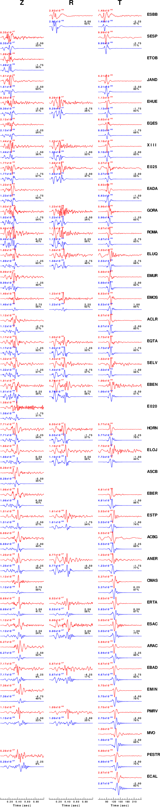
Figure 2. Depth sensitivity for waveform mechanism

The comparison of the observed and predicted waveforms is given in the next figure. The red traces are the observed and the blue are the predicted. Each observed-predicted component is plotted to the same scale and peak amplitudes are indicated by the numbers to the left of each trace. A pair of numbers is given in black at the right of each predicted traces. The upper number it the time shift required for maximum correlation between the observed and predicted traces. This time shift is required because the synthetics are not computed at exactly the same distance as the observed and because the velocity model used in the predictions may not be perfect. A positive time shift indicates that the prediction is too fast and should be delayed to match the observed trace (shift to the right in this figure). A negative value indicates that the prediction is too slow. The lower number gives the percentage of variance reduction to characterize the individual goodness of fit (100% indicates a perfect fit).

The bandpass filter used in the processing and for the display was

hp c 0.02 n 3
lp c 0.06 n 3

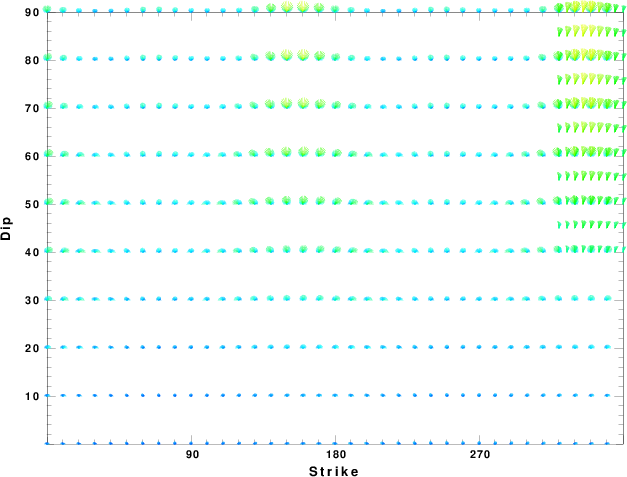
Figure 3. Waveform comparison for selected depth

Focal mechanism sensitivity at the preferred depth. The red color indicates a very good fit to thewavefroms. Each solution is plotted as a vector at a given value of strike and dip with the angle of the vector representing the rake angle, measured, with respect to the upward vertical (N) in the figure.

A check on the assumed source location is possible by looking at the time shifts between the observed and predicted traces. The time shifts for waveform matching arise for several reasons:

The origin time and epicentral distance are incorrect
The velocity model used for the inversion is incorrect
The velocity model used to define the P-arrival time is not the same as the velocity model used for the waveform inversion (assuming that the initial trace alignment is based on the P arrival time)

Assuming only a mislocation, the time shifts are fit to a functional form:

 Time_shift = A + B cos Azimuth + C Sin Azimuth

The time shifts for this inversion lead to the next figure:

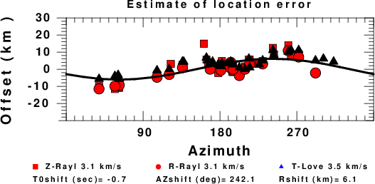
The derived shift in origin time and epicentral coordinates are given at the bottom of the figure.

Discussion

Acknowledgements

Thanks also to the many seismic network operators whose dedication make this effort possible: University of Nevada Reno, University of Alaska, University of Washington, Oregon State University, University of Utah, Montana Bureas of Mines, UC Berkely, Caltech, UC San Diego, Saint Louis University, University of Memphis, Lamont Doherty Earth Observatory, the Iris stations and the Transportable Array of EarthScope.

Velocity Model

The WUS used for the waveform synthetic seismograms and for the surface wave eigenfunctions and dispersion is as follows:

MODEL.01
Model after     8 iterations
ISOTROPIC
KGS
FLAT EARTH
1-D
CONSTANT VELOCITY
LINE08
LINE09
LINE10
LINE11
      H(KM)   VP(KM/S)   VS(KM/S) RHO(GM/CC)         QP         QS       ETAP       ETAS      FREFP      FREFS
     1.9000     3.4065     2.0089     2.2150  0.302E-02  0.679E-02   0.00       0.00       1.00       1.00    
     6.1000     5.5445     3.2953     2.6089  0.349E-02  0.784E-02   0.00       0.00       1.00       1.00    
    13.0000     6.2708     3.7396     2.7812  0.212E-02  0.476E-02   0.00       0.00       1.00       1.00    
    19.0000     6.4075     3.7680     2.8223  0.111E-02  0.249E-02   0.00       0.00       1.00       1.00    
     0.0000     7.9000     4.6200     3.2760  0.164E-10  0.370E-10   0.00       0.00       1.00       1.00

Quality Control

Here we tabulate the reasons for not using certain digital data sets

The following stations did not have a valid response files:

Last Changed Wed May 23 04:46:15 CDT 2012