Location
2007/08/12 07:47:05 39.36N -2.95.01W 5 4.7 Spain
Arrival Times (from USGS)
Arrival time list
Felt Map
USGS Felt map for this earthquake
USGS Felt reports page for Spain
Focal Mechanism
 SLU Moment Tensor Solution
 2007/08/12 07:47:05 39.36N -2.95.01W 5 4.7 Spain

 Best Fitting Double Couple
    Mo = 9.02e+22 dyne-cm
    Mw = 4.57
    Z  = 12 km
     Plane   Strike  Dip  Rake
      NP1       66    76   164
      NP2      160    75    15
 Principal Axes:
   Axis    Value   Plunge  Azimuth
     T   9.02e+22     21      23
     N   0.00e+00     69     204
     P  -9.02e+22      0     113


 Moment Tensor: (dyne-cm)
    Component  Value
       Mxx     5.27e+22
       Mxy     6.07e+22
       Mxz     2.81e+22
       Myy    -6.44e+22
       Myz     1.13e+22
       Mzz     1.17e+22


                     ##############
                 ----############   ###
              -------############ T ######
             --------############   #######
           ----------########################
          -----------#########################
         -------------#########################
        --------------#######################---
        ---------------####################-----
       ----------------##################--------
       -----------------##############-----------
       -----------------###########--------------
       ------------------######------------------
        ------------------#---------------------
        -------------#####-------------------
         ----##############------------------ P
          ##################-----------------
           ##################----------------
             #################-------------
              ##################----------
                 ################------
                     ##############


 Harvard Convention
 Moment Tensor:
      R          T          F
  1.17e+22   2.81e+22  -1.13e+22
  2.81e+22   5.27e+22  -6.07e+22
 -1.13e+22  -6.07e+22  -6.44e+22


Details of the solution is found at

http://www.eas.slu.edu/Earthquake_Center/MECH.EU/20070812074705/index.html
|
IGN (Madrid) Solution http://www.ign.es/ign/home/geofisica/sismologia/principalTensorUltimo.jsp?registros=91&inicio=1&fin=0&i=90
Evid  	Fecha  	Hora  	Latitud  	Longitud  	Prof  	Mw  	Localización
780720 	12/08/2007 	07:47:05 	39.357 	-2.986 	9 	4.7 	SW PEDRO MUQOZ.CR
|
Preferred Solution
The preferred solution from an analysis of the surface-wave spectral amplitude radiation pattern, waveform inversion and first motion observations is
      STK = 160
      DIP = 75
     RAKE = 15
       MW = 4.57
       HS = 12
The waveform inversion is preferred.
Waveform Inversion
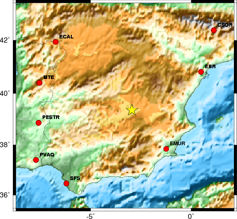
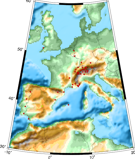
The focal mechanism was determined using broadband seismic waveforms. The location of the event and the
and stations used for the waveform inversion are shown in the next figure.
|
|
Location of broadband stations used for waveform inversion
|
The program wvfgrd96 was used with good traces observed at short distance to determine the focal mechanism, depth and seismic moment. This technique requires a high quality signal and well determined velocity model for the Green functions. To the extent that these are the quality data, this type of mechanism should be preferred over the radiation pattern technique which requires the separate step of defining the pressure and tension quadrants and the correct strike.
The observed and predicted traces are filtered using the following gsac commands:
hp c 0.02 n 4
lp c 0.10 n 4
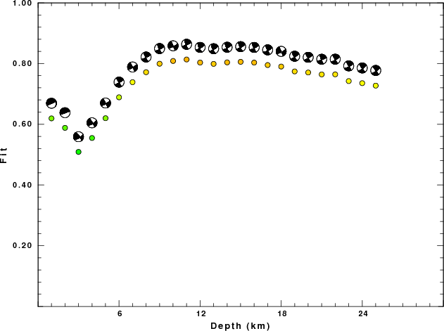
The results of this grid search from 0.5 to 19 km depth are as follow:
           DEPTH  STK   DIP  RAKE   MW    FIT
WVFGRD96    0.5   250    65    35   4.29 0.2643
WVFGRD96    1.0   255    55    35   4.33 0.2734
WVFGRD96    2.0   255    60    35   4.38 0.2986
WVFGRD96    3.0   260    55    40   4.43 0.3050
WVFGRD96    4.0   160    80    20   4.39 0.3006
WVFGRD96    5.0   160    75    20   4.42 0.3143
WVFGRD96    6.0   160    70    20   4.44 0.3268
WVFGRD96    7.0   160    70    15   4.47 0.3388
WVFGRD96    8.0   160    70    20   4.51 0.3497
WVFGRD96    9.0   160    70    15   4.53 0.3582
WVFGRD96   10.0   160    75    15   4.54 0.3641
WVFGRD96   11.0   160    75    15   4.56 0.3673
WVFGRD96   12.0   160    75    15   4.57 0.3683
WVFGRD96   13.0   155    80    15   4.58 0.3676
WVFGRD96   14.0   160    80    10   4.60 0.3650
WVFGRD96   15.0   340    80    10   4.62 0.3616
WVFGRD96   16.0   340    80    10   4.63 0.3577
WVFGRD96   17.0   340    80    10   4.64 0.3520
WVFGRD96   18.0   340    80    10   4.65 0.3448
WVFGRD96   19.0   340    80    10   4.66 0.3365
WVFGRD96   20.0   340    80    10   4.67 0.3265
WVFGRD96   21.0   340    80    10   4.67 0.3156
WVFGRD96   22.0   340    80    10   4.68 0.3037
WVFGRD96   23.0   340    80    10   4.68 0.2923
WVFGRD96   24.0   340    80    10   4.69 0.2807
WVFGRD96   25.0   340    80    10   4.69 0.2682
WVFGRD96   26.0   340    85    10   4.69 0.2560
WVFGRD96   27.0   340    90    15   4.69 0.2440
WVFGRD96   28.0   155    40   -20   4.73 0.2396
WVFGRD96   29.0   160    40   -15   4.74 0.2353
The best solution is
WVFGRD96 12.0 160 75 15 4.57 0.3683
The mechanism correspond to the best fit is
|
|
Figure 1. Waveform inversion focal mechanism
|
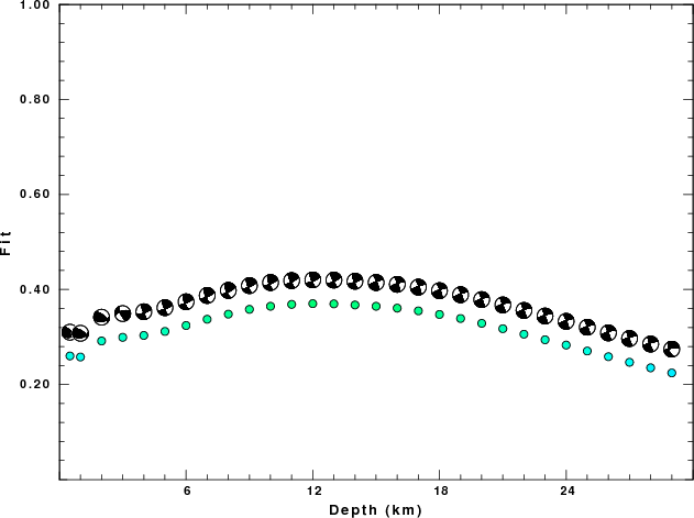
The best fit as a function of depth is given in the following figure:
|
|
Figure 2. Depth sensitivity for waveform mechanism
|
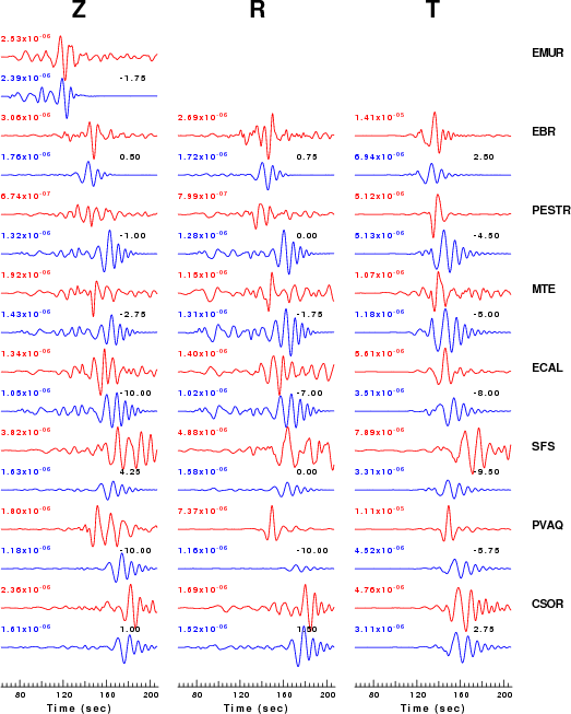
The comparison of the observed and predicted waveforms is given in the next figure. The red traces are the observed and the blue are the predicted.
Each observed-predicted componnet is plotted to the same scale and peak amplitudes are indicated by the numbers to the left of each trace. The number in black at the rightr of each predicted traces it the time shift required for maximum correlation between the observed and predicted traces. This time shift is required because the synthetics are not computed at exactly the same distance as the observed and because the velocity model used in the predictions may not be perfect.
A positive time shift indicates that the prediction is too fast and should be delayed to match the observed trace (shift to the right in this figure). A negative value indicates that the prediction is too slow.
The bandpass filter used in the processing and for the display was
hp c 0.02 n 4
lp c 0.10 n 4
|
|
Figure 3. Waveform comparison for depth of 8 km
|
|
|
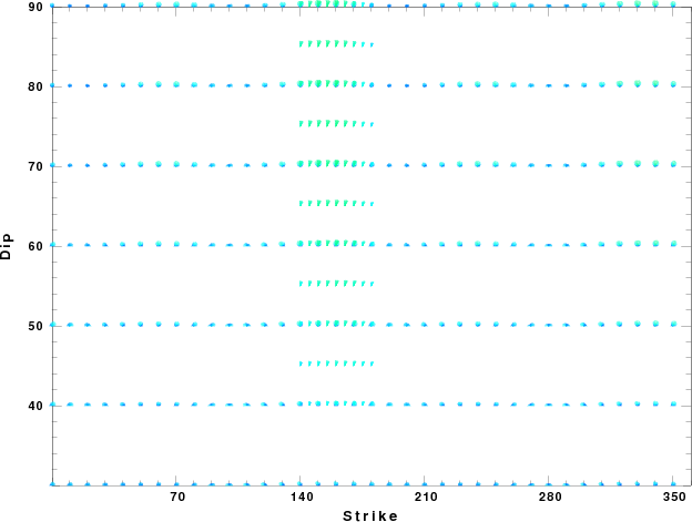
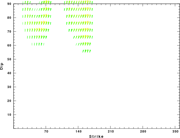
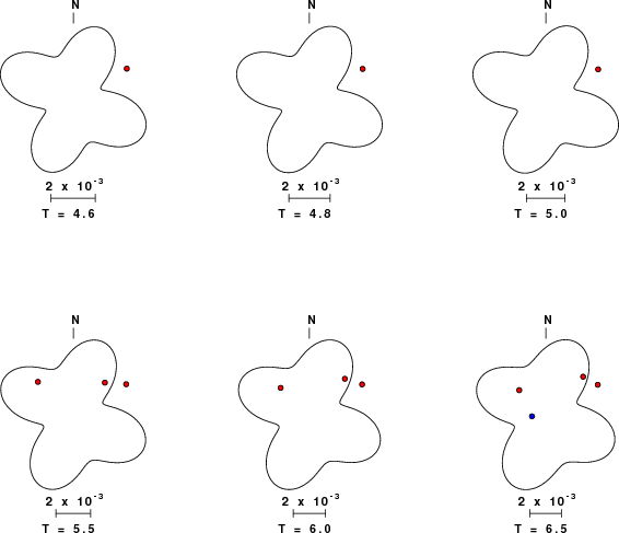
Focal mechanism sensitivity at the preferred depth. The red color indicates a very good fit to thewavefroms.
Each solution is plotted as a vector at a given value of strike and dip with the angle of the vector representing the rake angle, measured, with respect to the upward vertical (N) in the figure.
|
Surface-Wave Focal Mechanism
The following figure shows the stations used in the grid search for the best focal mechanism to fit the surface-wave spectral amplitudes of the Love and Rayleigh waves.
|
|
Location of broadband stations used to obtain focal mechanism from surface-wave spectral amplitudes
|
The surface-wave determined focal mechanism is shown here.
  NODAL PLANES


  STK=      67.38
  DIP=      80.34
 RAKE=     164.78

             OR

  STK=     159.99
  DIP=      75.00
 RAKE=      10.00


DEPTH = 11.0 km

Mw = 4.75
Best Fit 0.8134 - P-T axis plot gives solutions with FIT greater than FIT90
First motion data
The P-wave first motion data for focal mechanism studies are as follow:
Sta Az(deg) Dist(km) First motion
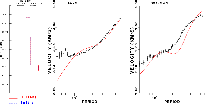
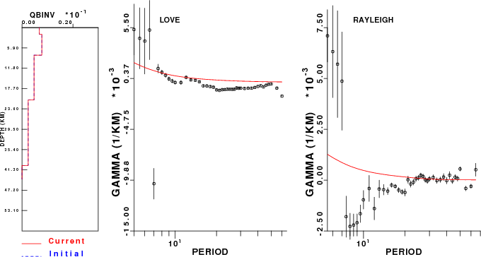
Surface-wave analysis
Surface wave analysis was performed using codes from
Computer Programs in Seismology, specifically the
multiple filter analysis program do_mft and the surface-wave
radiation pattern search program srfgrd96.
Data preparation
Digital data were collected, instrument response removed and traces converted
to Z, R an T components. Multiple filter analysis was applied to the Z and T traces to obtain the Rayleigh- and Love-wave spectral amplitudes, respectively.
These were input to the search program which examined all depths between 1 and 25 km
and all possible mechanisms.
|
|
Best mechanism fit as a function of depth. The preferred depth is given above. Lower hemisphere projection
|
|
|
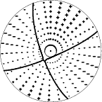
Pressure-tension axis trends. Since the surface-wave spectra search does not distinguish between P and T axes and since there is a 180 ambiguity in strike, all possible P and T axes are plotted. First motion data and waveforms will be used to select the preferred mechanism. The purpose of this plot is to provide an idea of the
possible range of solutions. The P and T-axes for all mechanisms with goodness of fit greater than 0.9 FITMAX (above) are plotted here.
|
|
|
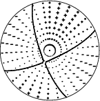
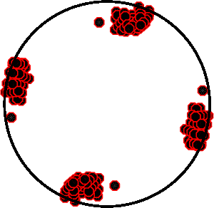
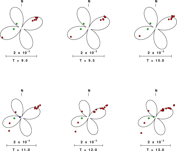
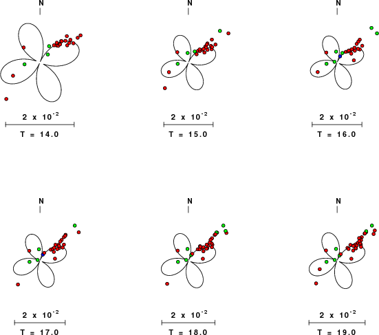
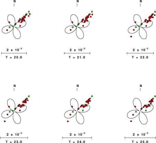
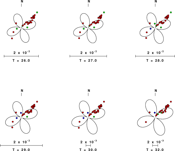
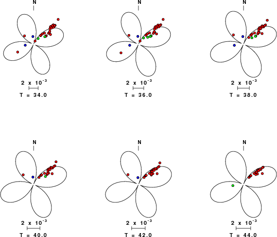
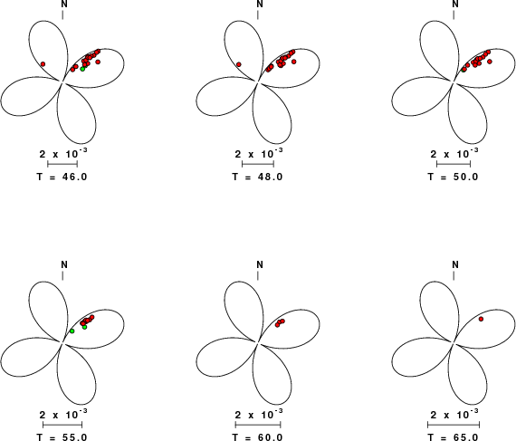
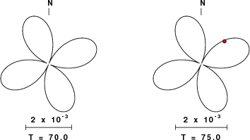
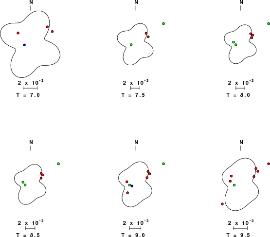
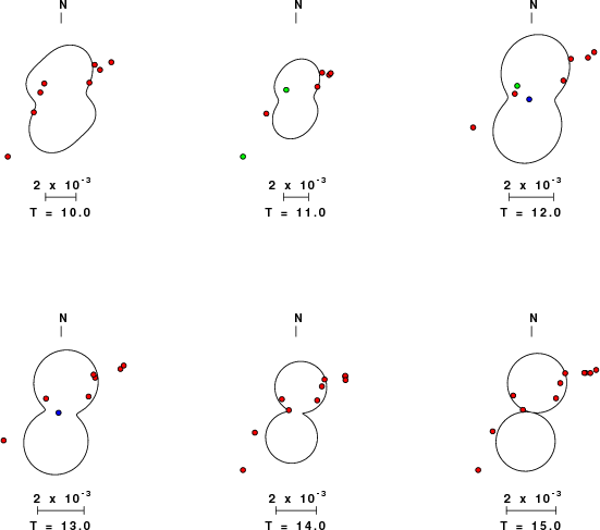
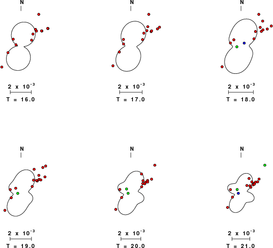
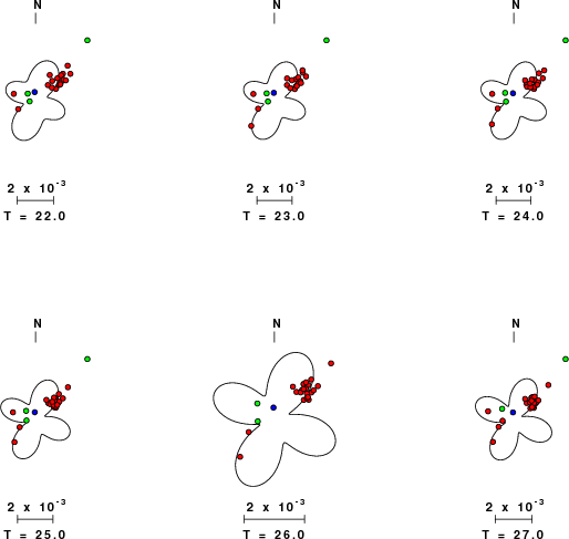
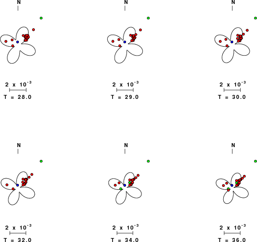
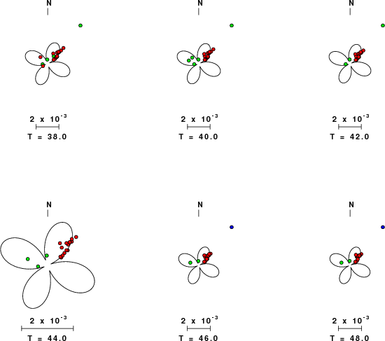
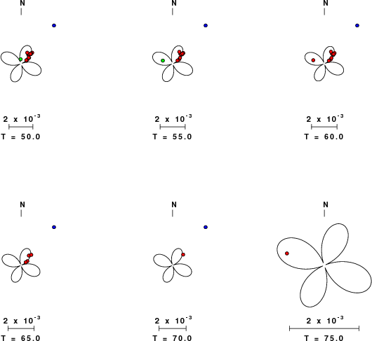
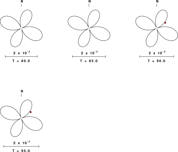
Focal mechanism sensitivity at the preferred depth. The red color indicates a very good fit to the Love and Rayleigh wave radiation patterns.
Each solution is plotted as a vector at a given value of strike and dip with the angle of the vector representing the rake angle, measured, with respect to the upward vertical (N) in the figure. Because of the symmetry of the spectral amplitude rediation patterns, only strikes from 0-180 degrees are sampled.
|
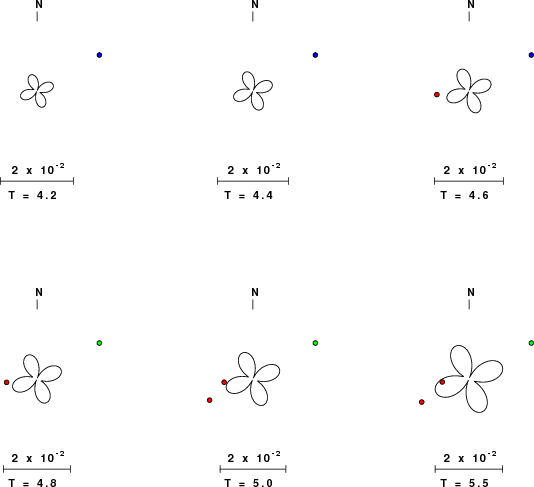
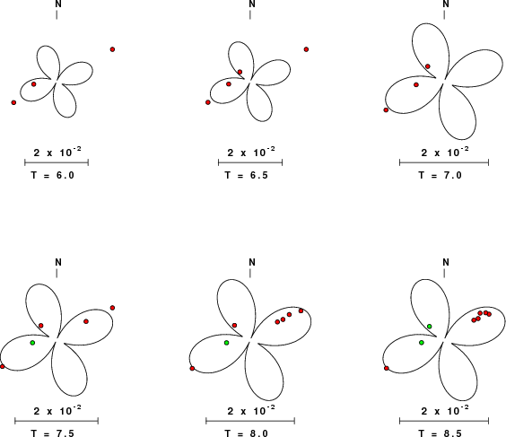
Love-wave radiation patterns
Rayleigh-wave radiation patterns
Broadband station distribution
The distribution of broadband stations with azimuth and distance is
Sta Az(deg)    Dist(km)
EBR	   60	  335
PESTR	  264	  405
MTE	  288	  410
ECAL	  313	  430
SFS	  223	  430
PVAQ	  244	  470
CSOR	   44	  480
EJON	   53	  599
MAHO	   82	  622
ARBF	   54	  830
RUSF	   51	  867
SSB	   41	  901
OGDI	   52	  927
CALF	   56	  956
ANTI	   58	  961
ESCA	   57	  993
SAOF	   56	 1013
GIMEL	   40	 1094
EMV	   44	 1097
AIGLE	   43	 1120
DIX	   45	 1129
BRANT	   39	 1137
SENIN	   44	 1141
MMK	   47	 1161
BOURR	   39	 1214
HASLI	   44	 1220
MUGIO	   50	 1222
FUSIO	   46	 1231
MUO	   44	 1264
LLS	   46	 1278
VDL	   48	 1282
ZUR	   43	 1288
HTL	  355	 1298
PLONS	   46	 1314
BERNI	   49	 1315
DAVOX	   48	 1328
LIENZ	   45	 1337
FUORN	   49	 1343
BFO	   38	 1345
WLF	   29	 1352
DAVA	   46	 1360
HGN	   26	 1445
WTTA	   49	 1470
FUR	   45	 1502
Waveform comparison for this mechanism
Since the analysis of the surface-wave radiation patterns uses only spectral
amplitudes and because the surfave-wave radiation patterns have a 180 degree symmetry, each surface-wave solution consists of four possible focal mechanisms corresponding to the interchange of the P- and T-axes and a roation of the mechanism by 180 degrees. To select one mechanism, P-wave first motion can be used. This was not possible in this case because all the P-wave first motions were
emergent ( a feature of the P-wave wave takeoff angle, the station location and the mechanism). The other way to select among the mechanisms is to compute
forward synthetics and compare the observed and predicted waveforms.
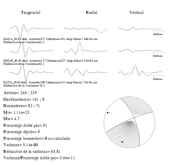
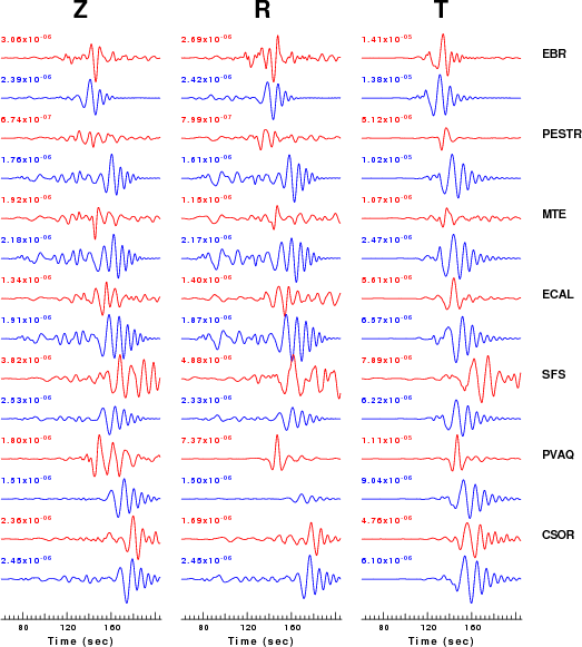
The fits to the waveforms with the given mechanism are show below:
This figure shows the fit to the three components of motion (Z - vertical, R-radial and T - transverse). For each station and component, the
observed traces is shown in red and the model predicted trace in blue. The traces represent filtered ground velocity in units of meters/sec (the peak value is printed adjacent to each trace; each pair of traces to plotted to the same scale to emphasize the difference in levels). Both synthetic and observed traces have been filtered using the SAC commands:
hp c 0.02 n 4
lp c 0.10 n 4
Discussion
The Future
Should the national backbone of the
USGS Advanced National Seismic System (ANSS)
be implemented with an interstation separation of 300 km, it is very likely that
an earthquake such as this would have been recorded at distances on the order of
100-200 km. This means that the closest station would have information on
source depth and mechanism that was lacking here.
Acknowledgements
Dr. Harley Benz, USGS, provided the USGS USNSN digital data.
The digital data used in this study were provided by Natural Resources Canada through their AUTODRM site http://www.seismo.nrcan.gc.ca/nwfa/autodrm/autodrm_req_e.php, and IRIS using their BUD interface
Appendix A
Spectra fit plots to each station
Velocity Model
The WUS used for the waveform synthetic seismograms and for the surface wave eigenfunctions and dispersion is as follows:
MODEL.01
Model after     8 iterations
ISOTROPIC
KGS
FLAT EARTH
1-D
CONSTANT VELOCITY
LINE08
LINE09
LINE10
LINE11
      H(KM)   VP(KM/S)   VS(KM/S) RHO(GM/CC)         QP         QS       ETAP       ETAS      FREFP      FREFS
     1.9000     3.4065     2.0089     2.2150  0.302E-02  0.679E-02   0.00       0.00       1.00       1.00
     6.1000     5.5445     3.2953     2.6089  0.349E-02  0.784E-02   0.00       0.00       1.00       1.00
    13.0000     6.2708     3.7396     2.7812  0.212E-02  0.476E-02   0.00       0.00       1.00       1.00
    19.0000     6.4075     3.7680     2.8223  0.111E-02  0.249E-02   0.00       0.00       1.00       1.00
     0.0000     7.9000     4.6200     3.2760  0.164E-10  0.370E-10   0.00       0.00       1.00       1.00
Quality Control
Here we tabulate the reasons for not using certain digital data sets
The following stations did not have a valid response files:
DATE=Thu Aug 16 08:34:04 CDT 2007
Last Changed 2007/08/12