2006/11/17 18:19:50 43.12N 0.08E 10 4.6 France
USGS Felt map for this earthquake
USGS Felt reports page for Pyrenees, France
 SLU Moment Tensor Solution
 2006/11/17 18:19:50 43.12N 0.08E 10 4.6 France

 Best Fitting Double Couple
    Mo = 4.37e+22 dyne-cm
    Mw = 4.36
    Z  = 12 km
     Plane   Strike  Dip  Rake
      NP1      255    74   -127
      NP2      145    40   -25
 Principal Axes:
   Axis    Value   Plunge  Azimuth
     T   4.37e+22     20      12
     N   0.00e+00     36     266
     P  -4.37e+22     47     126


 Moment Tensor: (dyne-cm)
    Component  Value
       Mxx     2.99e+22
       Mxy     1.72e+22
       Mxz     2.67e+22
       Myy    -1.17e+22
       Myz    -1.48e+22
       Mzz    -1.82e+22


                     ##############
                 #############   ######
              -############### T #########
             --###############   ##########
           ---###############################
          ----################################
         ----##################################
        -----###################################
        -----#################------------------
       -------#########--------------------------
       -------####-------------------------------
       -------#----------------------------------
       ----####----------------------------------
        -#######-------------------   ----------
        #########------------------ P ----------
         ##########----------------   ---------
          ##########--------------------------
           ###########-----------------------
             ############------------------
              ##############--------------
                 ######################
                     ##############


 Harvard Convention
 Moment Tensor:
      R          T          F
 -1.82e+22   2.67e+22   1.48e+22
  2.67e+22   2.99e+22  -1.72e+22
  1.48e+22  -1.72e+22  -1.17e+22


Details of the solution is found at

http://www.eas.slu.edu/Earthquake_Center/MECH.NA/20061117181951/index.html
|
      STK = 145
      DIP = 40
     RAKE = -25
       MW = 4.36
       HS = 12
The waveform inversion is preferred. The surface-wave solution is in general agreement
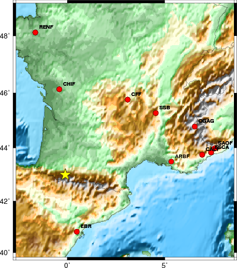
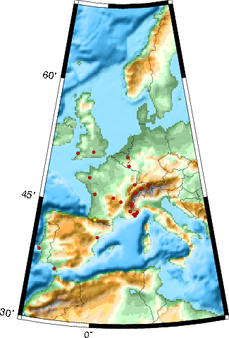
The focal mechanism was determined using broadband seismic waveforms. The location of the event and the and stations used for the waveform inversion are shown in the next figure.
|
|
|
|
The program wvfgrd96 was used with good traces observed at short distance to determine the focal mechanism, depth and seismic moment. This technique requires a high quality signal and well determined velocity model for the Green functions. To the extent that these are the quality data, this type of mechanism should be preferred over the radiation pattern technique which requires the separate step of defining the pressure and tension quadrants and the correct strike.
The observed and predicted traces are filtered using the following gsac commands:
hp c 0.02 n 3
lp c 0.06 n 3
br c 0.12 0.2 n 4 p 2
The results of this grid search from 0.5 to 19 km depth are as follow:
           DEPTH  STK   DIP  RAKE   MW    FIT
WVFGRD96    0.5   200    65    30   4.14 0.4188
WVFGRD96    1.0   195    75    25   4.13 0.4048
WVFGRD96    2.0   200    75    35   4.21 0.4375
WVFGRD96    3.0   200    80    45   4.27 0.4299
WVFGRD96    4.0   150    30   -10   4.33 0.4606
WVFGRD96    5.0   145    30   -20   4.34 0.4961
WVFGRD96    6.0   145    30   -20   4.35 0.5142
WVFGRD96    7.0   140    35   -30   4.35 0.5263
WVFGRD96    8.0   140    35   -30   4.37 0.5341
WVFGRD96    9.0   140    35   -30   4.37 0.5406
WVFGRD96   10.0   145    35   -25   4.36 0.5448
WVFGRD96   11.0   145    35   -25   4.36 0.5480
WVFGRD96   12.0   145    40   -25   4.36 0.5503
WVFGRD96   13.0   145    40   -25   4.36 0.5489
WVFGRD96   14.0   150    45   -15   4.35 0.5472
WVFGRD96   15.0   160    50    20   4.36 0.5479
WVFGRD96   16.0   160    50    20   4.36 0.5451
WVFGRD96   17.0   155    55    15   4.37 0.5429
WVFGRD96   18.0   155    55    15   4.38 0.5412
WVFGRD96   19.0   155    55    15   4.38 0.5359
WVFGRD96   20.0   155    60    20   4.39 0.5323
WVFGRD96   21.0   160    50    20   4.42 0.5236
WVFGRD96   22.0   160    50    20   4.43 0.5175
WVFGRD96   23.0   160    50    20   4.43 0.5116
WVFGRD96   24.0   160    55    20   4.44 0.5035
WVFGRD96   25.0   160    55    20   4.44 0.4965
WVFGRD96   26.0   160    55    20   4.45 0.4892
WVFGRD96   27.0   160    55    20   4.46 0.4801
WVFGRD96   28.0   160    55    20   4.46 0.4714
WVFGRD96   29.0   160    55    20   4.47 0.4622
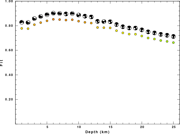
The best solution is
WVFGRD96 12.0 145 40 -25 4.36 0.5503
The mechanism correspond to the best fit is
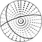
|
|
|
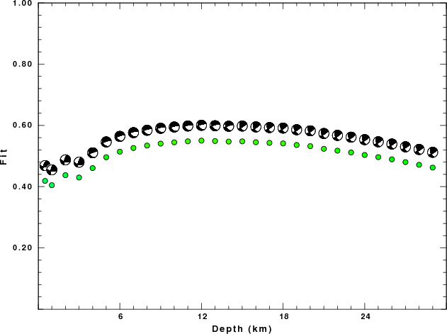
The best fit as a function of depth is given in the following figure:
|
|
|
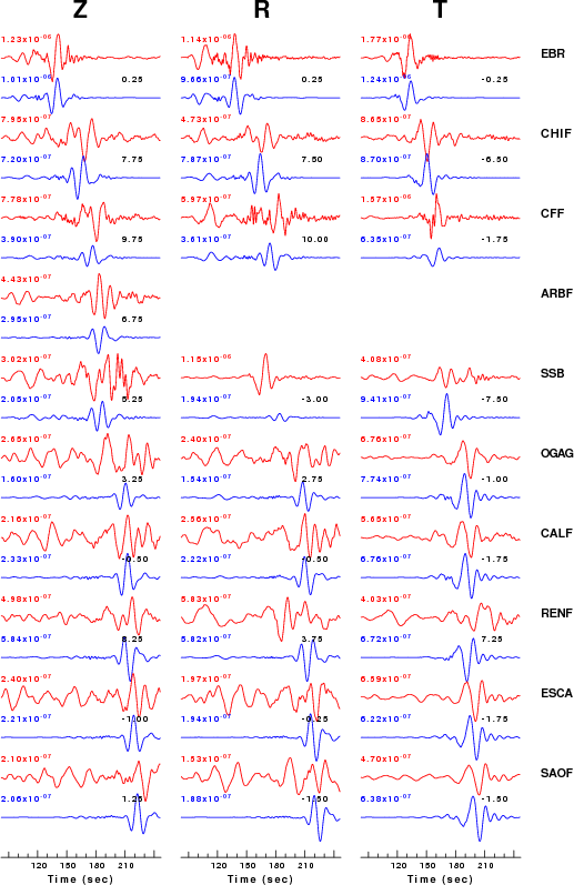
The comparison of the observed and predicted waveforms is given in the next figure. The red traces are the observed and the blue are the predicted. Each observed-predicted componnet is plotted to the same scale and peak amplitudes are indicated by the numbers to the left of each trace. The number in black at the rightr of each predicted traces it the time shift required for maximum correlation between the observed and predicted traces. This time shift is required because the synthetics are not computed at exactly the same distance as the observed and because the velocity model used in the predictions may not be perfect. A positive time shift indicates that the prediction is too fast and should be delayed to match the observed trace (shift to the right in this figure). A negative value indicates that the prediction is too slow. The bandpass filter used in the processing and for the display was
hp c 0.02 n 3
lp c 0.06 n 3
br c 0.12 0.2 n 4 p 2
|
|
|
|
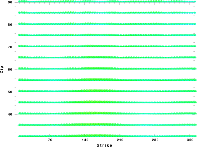
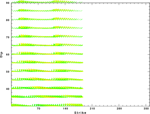
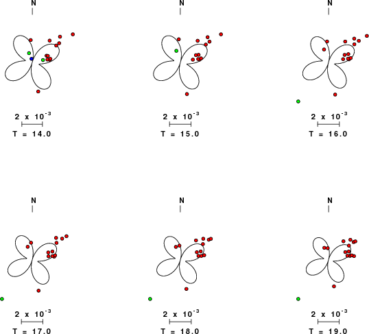
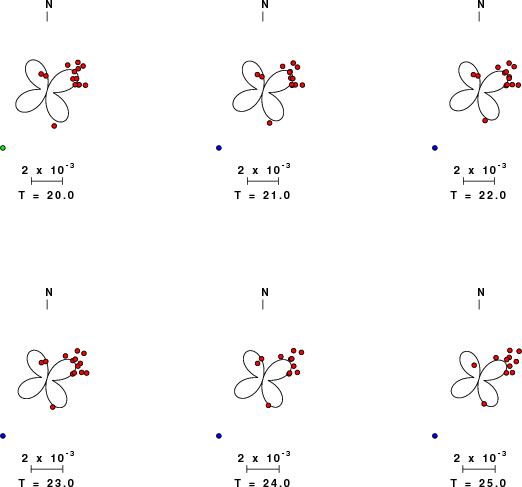
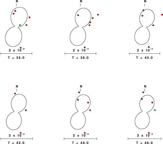
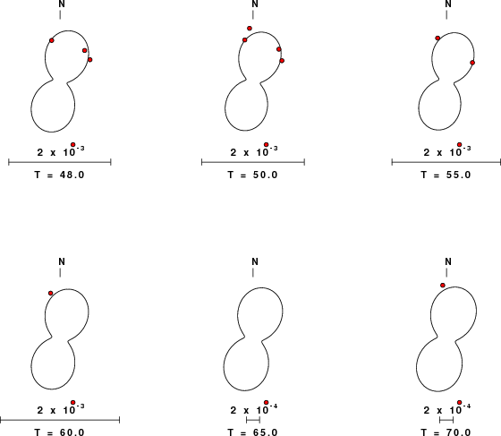
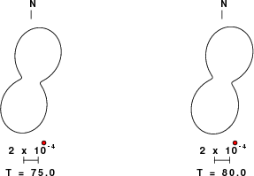
| Focal mechanism sensitivity at the preferred depth. The red color indicates a very good fit to thewavefroms. Each solution is plotted as a vector at a given value of strike and dip with the angle of the vector representing the rake angle, measured, with respect to the upward vertical (N) in the figure. |
The following figure shows the stations used in the grid search for the best focal mechanism to fit the surface-wave spectral amplitudes of the Love and Rayleigh waves.
|
|
|
The surface-wave determined focal mechanism is shown here.
  NODAL PLANES


  STK=     284.99
  DIP=      55.00
 RAKE=     -90.01

             OR

  STK=     105.00
  DIP=      35.00
 RAKE=     -89.99


DEPTH = 6.0 km

Mw = 4.48
Best Fit 0.8522 - P-T axis plot gives solutions with FIT greater than FIT90
 |
The P-wave first motion data for focal mechanism studies are as follow:
Sta Az(deg)    Dist(km)   First motion
EBR       168  247 eP_+
CHIF      356  349 iP_D
CFF        39  399 eP_X
ARBF       81  445 eP_X
SSB        54  450 eP_X
OGAG       67  569 eP_X
CALF       79  575 eP_X
RENF      349  582 eP_X
ESCA       79  612 eP_X
SAOF       77  629 eP_X
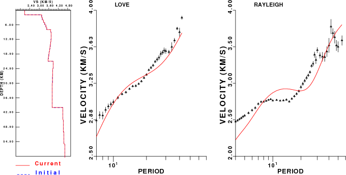
Surface wave analysis was performed using codes from Computer Programs in Seismology, specifically the multiple filter analysis program do_mft and the surface-wave radiation pattern search program srfgrd96.
The velocity model used for the search is a modified Utah model .
Digital data were collected, instrument response removed and traces converted
to Z, R an T components. Multiple filter analysis was applied to the Z and T traces to obtain the Rayleigh- and Love-wave spectral amplitudes, respectively.
These were input to the search program which examined all depths between 1 and 25 km
and all possible mechanisms.
|
|
|

|
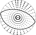
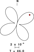
| Pressure-tension axis trends. Since the surface-wave spectra search does not distinguish between P and T axes and since there is a 180 ambiguity in strike, all possible P and T axes are plotted. First motion data and waveforms will be used to select the preferred mechanism. The purpose of this plot is to provide an idea of the possible range of solutions. The P and T-axes for all mechanisms with goodness of fit greater than 0.9 FITMAX (above) are plotted here. |
|
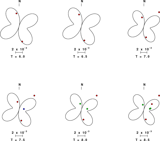
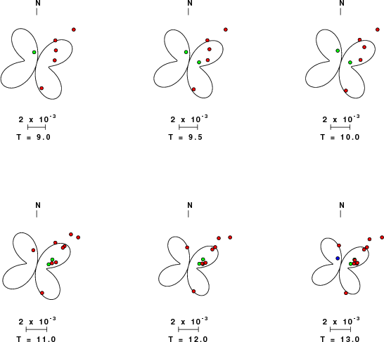
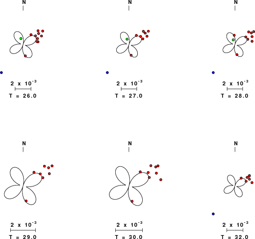
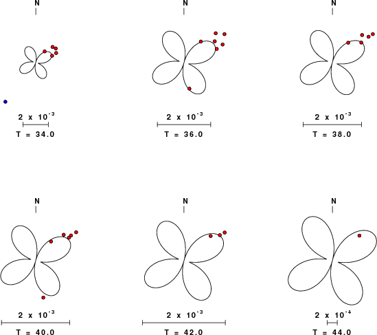
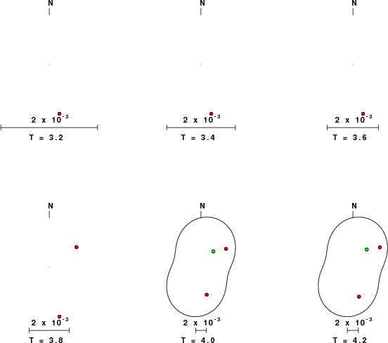
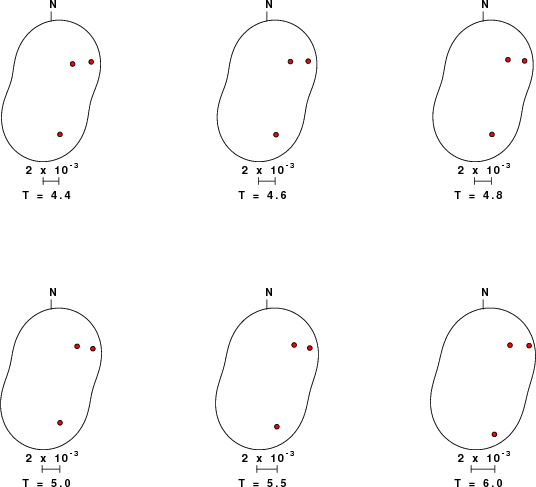
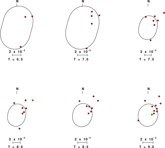
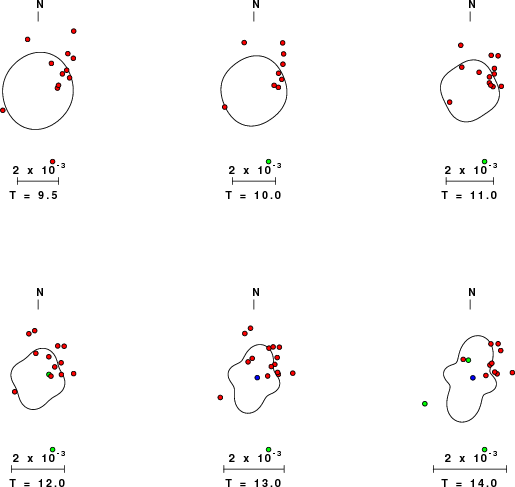
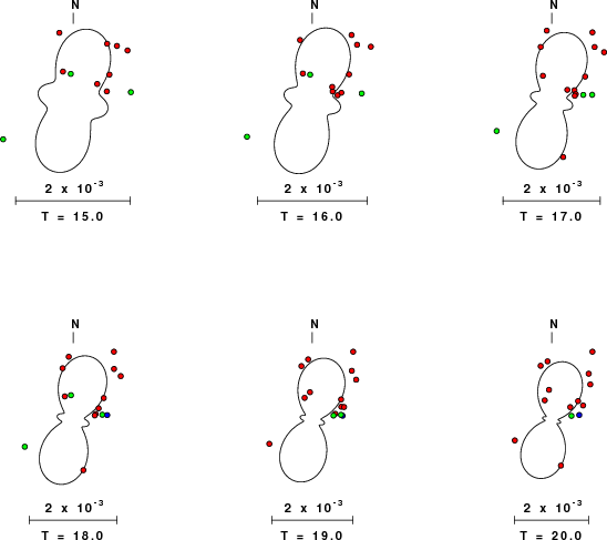
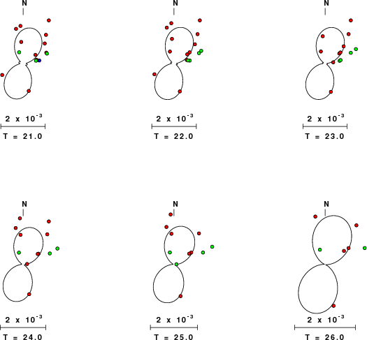
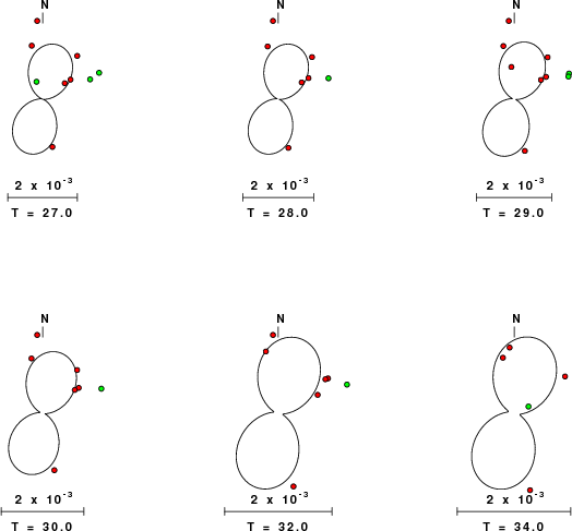
| Focal mechanism sensitivity at the preferred depth. The red color indicates a very good fit to the Love and Rayleigh wave radiation patterns. Each solution is plotted as a vector at a given value of strike and dip with the angle of the vector representing the rake angle, measured, with respect to the upward vertical (N) in the figure. Because of the symmetry of the spectral amplitude rediation patterns, only strikes from 0-180 degrees are sampled. |
Sta Az(deg)    Dist(km)
EBR	  168	  247
CHIF	  356	  349
CFF	   39	  399
SSB	   54	  450
OGDI	   74	  526
OGAG	   67	  569
CALF	   79	  575
RENF	  349	  582
BNI	   65	  589
ANTI	   81	  590
ESCA	   79	  612
SAOF	   77	  629
SENIN	   55	  695
BOURR	   47	  755
BNALP	   54	  799
WLF	   31	  883
SFS	  218	  894
PMST	  241	  900
DAVA	   55	  918
WOL	  355	  928
HTL	  341	  949
HGN	   26	  978
Since the analysis of the surface-wave radiation patterns uses only spectral amplitudes and because the surfave-wave radiation patterns have a 180 degree symmetry, each surface-wave solution consists of four possible focal mechanisms corresponding to the interchange of the P- and T-axes and a roation of the mechanism by 180 degrees. To select one mechanism, P-wave first motion can be used. This was not possible in this case because all the P-wave first motions were emergent ( a feature of the P-wave wave takeoff angle, the station location and the mechanism). The other way to select among the mechanisms is to compute forward synthetics and compare the observed and predicted waveforms.
The velocity model used for the waveform fit is a modified Utah model .
The fits to the waveforms with the given mechanism are show below:
|
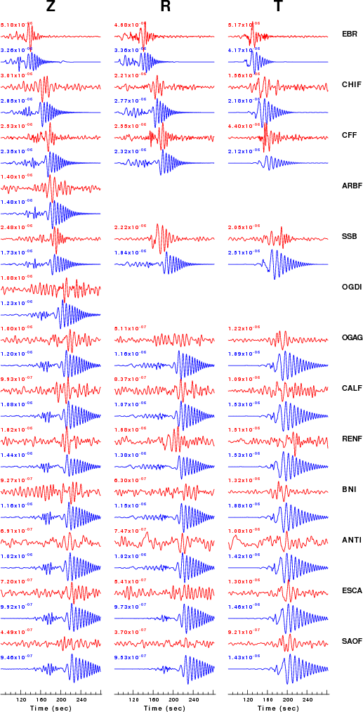
This figure shows the fit to the three components of motion (Z - vertical, R-radial and T - transverse). For each station and component, the observed traces is shown in red and the model predicted trace in blue. The traces represent filtered ground velocity in units of meters/sec (the peak value is printed adjacent to each trace; each pair of traces to plotted to the same scale to emphasize the difference in levels). Both synthetic and observed traces have been filtered using the SAC commands:
hp c 0.02 n 3
lp c 0.10 n 3
|
|
Should the national backbone of the USGS Advanced National Seismic System (ANSS) be implemented with an interstation separation of 300 km, it is very likely that an earthquake such as this would have been recorded at distances on the order of 100-200 km. This means that the closest station would have information on source depth and mechanism that was lacking here.
Dr. Harley Benz, USGS, provided the USGS USNSN digital data. The digital data used in this study were provided by Natural Resources Canada through their AUTODRM site http://www.seismo.nrcan.gc.ca/nwfa/autodrm/autodrm_req_e.php, and IRIS using their BUD interface
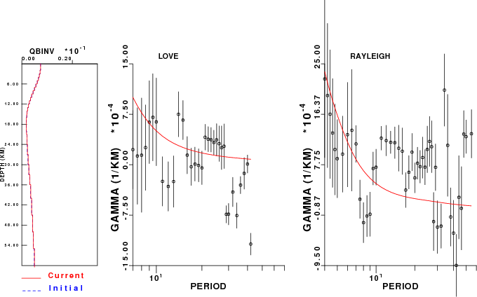
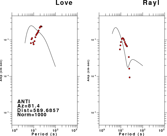
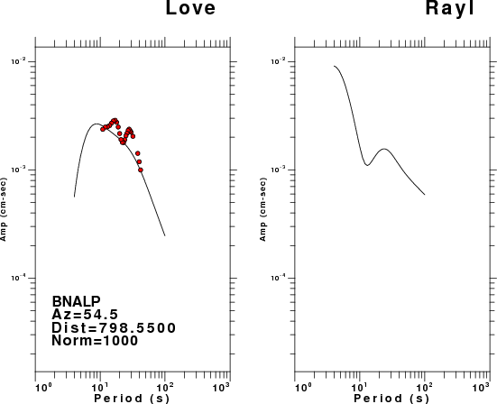
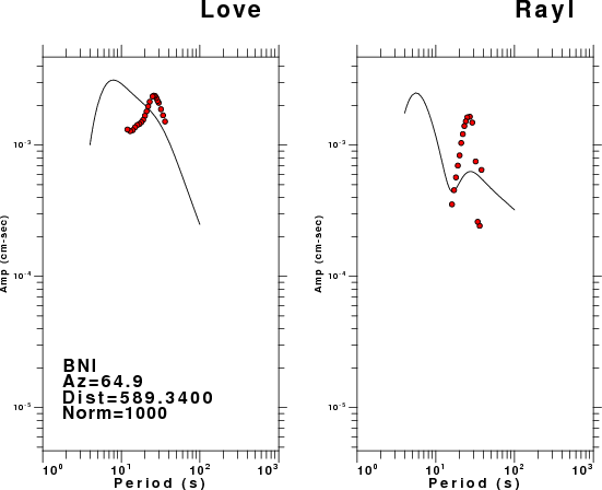
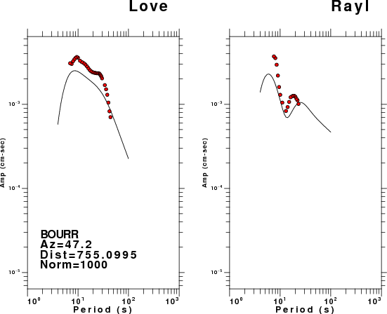
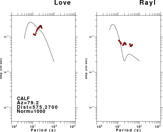
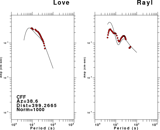
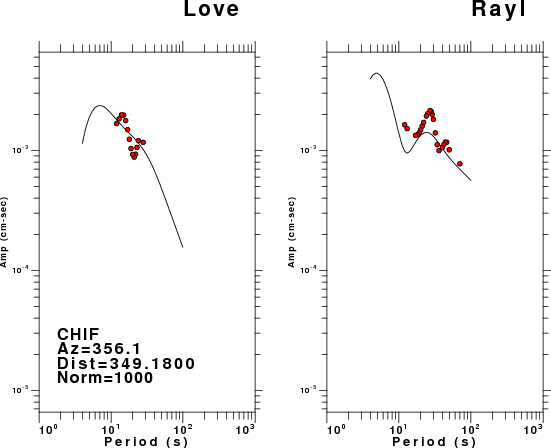
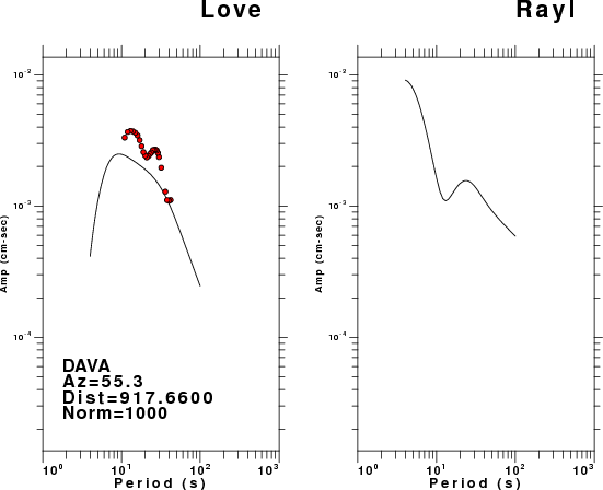
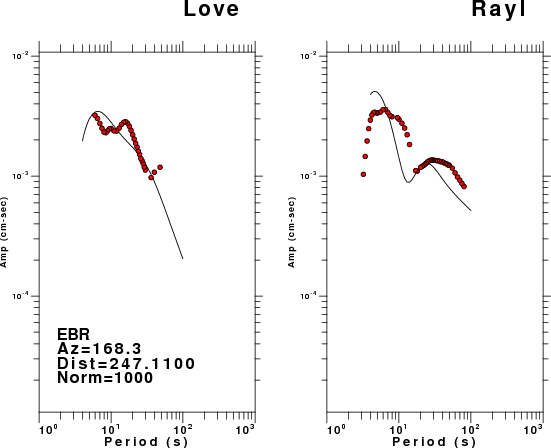
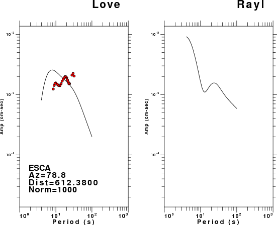
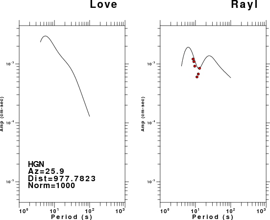
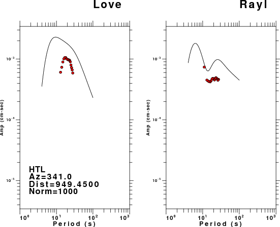
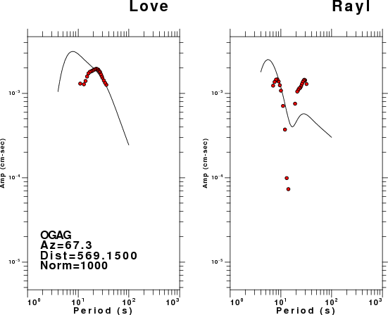
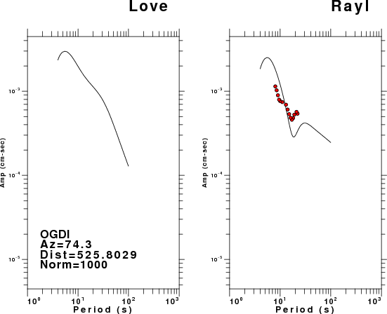
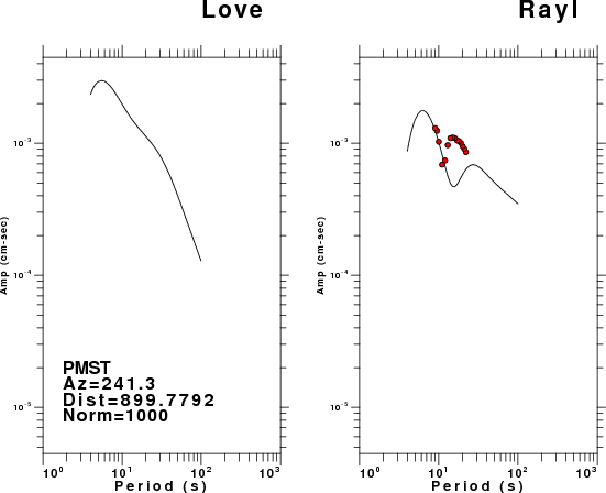
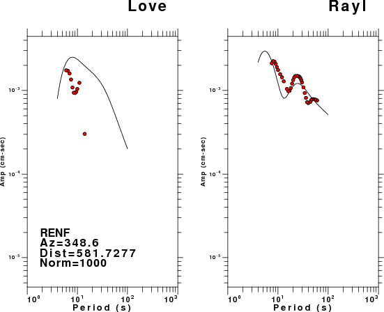
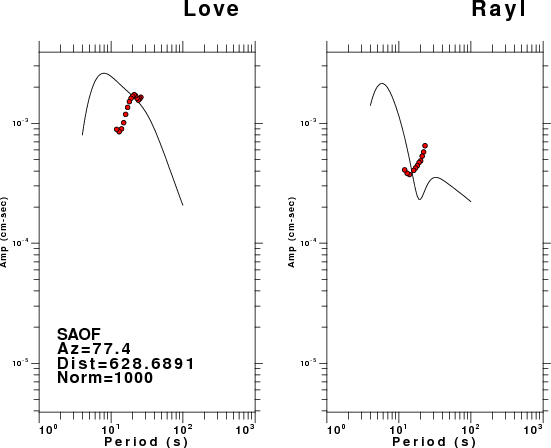
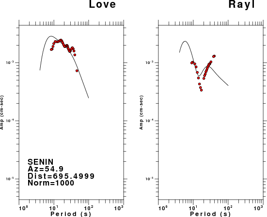
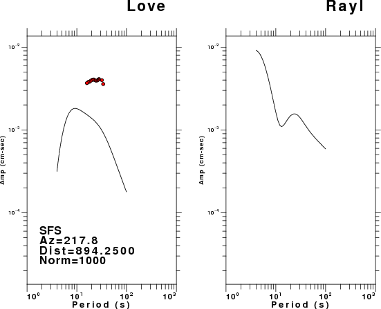
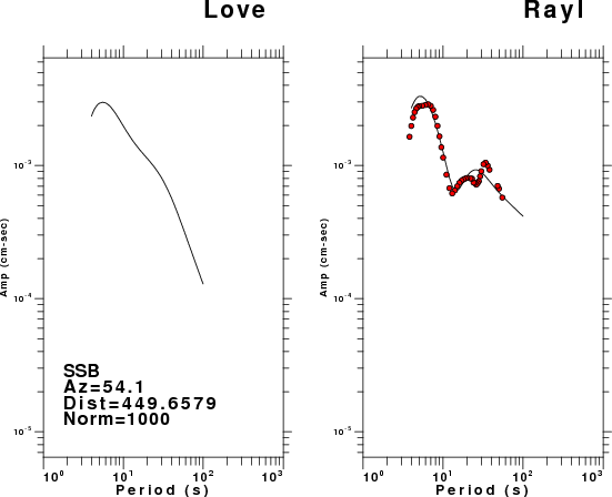
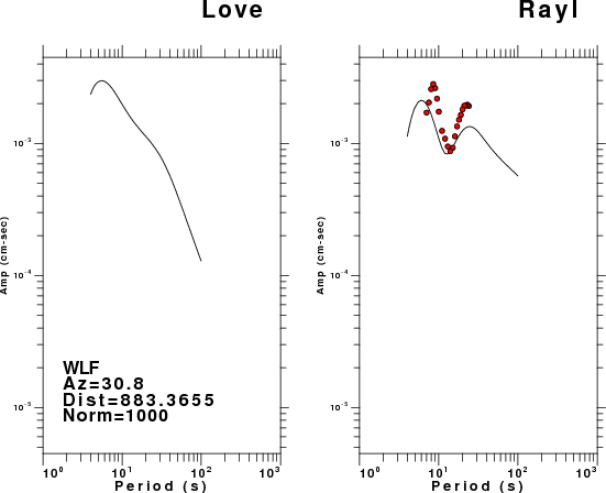
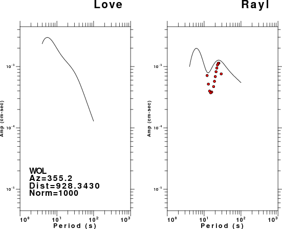
The figures below show the observed spectral amplitudes (units of cm-sec) at each station and the
theoretical predictions as a function of period for the mechanism given above. The modified Utah model earth model
was used to define the Green's functions. For each station, the Love and Rayleigh wave spectrail amplitudes are plotted with the same scaling so that one can get a sense fo the effects of the effects of the focal mechanism and depth on the excitation of each.
 |
 |
 |
 |
 |
 |
 |
 |
 |
 |
 |
 |
 |
 |
 |
 |
 |
 |
 |
 |
 |
 |
Here we tabulate the reasons for not using certain digital data sets
The following stations did not have a valid response files: