2004/02/24 05:21:26 15.43N 40.72E 10 4.0 Italy
USGS Felt map for this earthquake
 SLU Moment Tensor Solution
 2004/02/24 05:21:26 15.43N 40.72E 10 4.0 Italy

 Best Fitting Double Couple
    Mo = 1.50e+22 dyne-cm
    Mw = 4.05
    Z  = 12 km
     Plane   Strike  Dip  Rake
      NP1      288    68   -125
      NP2      170    40   -35
 Principal Axes:
   Axis    Value   Plunge  Azimuth
     T   1.50e+22     16      43
     N   0.00e+00     32     302
     P  -1.50e+22     53     156


 Moment Tensor: (dyne-cm)
    Component  Value
       Mxx     2.95e+21
       Mxy     8.85e+21
       Mxz     9.51e+21
       Myy     5.50e+21
       Myz    -1.63e+20
       Mzz    -8.45e+21


                     --############
                 ----##################
              -----#######################
             -----#####################   #
           ------###################### T ###
          -------######################   ####
         -------###############################
        ########---------#######################
        #######----------------#################
       ########---------------------#############
       ########------------------------##########
       #########--------------------------#######
       #########----------------------------#####
        ########------------------------------##
        #########-------------   ---------------
         #########------------ P --------------
          #########-----------   -------------
           #########-------------------------
             ########----------------------
              #########-------------------
                 ########--------------
                     #######-------


 Harvard Convention
 Moment Tensor:
      R          T          F
 -8.45e+21   9.51e+21   1.63e+20
  9.51e+21   2.95e+21  -8.85e+21
  1.63e+20  -8.85e+21   5.50e+21


Details of the solution is found at

http://www.eas.slu.edu/Earthquake_Center/MECH.NA/20040224052126/index.html
|
      STK = 170
      DIP = 40
     RAKE = -35
       MW = 4.05
       HS = 12
The focal mechanism was determined using broadband seismic waveforms. The location of the event and the and stations used for the waveform inversion are shown in the next figure.
|
|
|
|
The program wvfgrd96 was used with good traces observed at short distance to determine the focal mechanism, depth and seismic moment. This technique requires a high quality signal and well determined velocity model for the Green functions. To the extent that these are the quality data, this type of mechanism should be preferred over the radiation pattern technique which requires the separate step of defining the pressure and tension quadrants and the correct strike.
The observed and predicted traces are filtered using the following gsac commands:
hp c 0.02 n 3
lp c 0.10 n 3
The results of this grid search from 0.5 to 19 km depth are as follow:
           DEPTH  STK   DIP  RAKE   MW    FIT
WVFGRD96    0.5   270    30   100   3.67 0.2731
WVFGRD96    1.0   205    45    30   3.64 0.2690
WVFGRD96    2.0    60    55    90   3.80 0.3456
WVFGRD96    3.0   200    50    20   3.81 0.3689
WVFGRD96    4.0   185    25     0   3.87 0.4239
WVFGRD96    5.0   180    30   -15   3.90 0.4817
WVFGRD96    6.0   180    30   -15   3.92 0.5255
WVFGRD96    7.0   175    35   -25   3.95 0.5586
WVFGRD96    8.0   175    35   -25   3.99 0.5813
WVFGRD96    9.0   175    35   -25   4.01 0.5983
WVFGRD96   10.0   170    35   -35   4.03 0.6075
WVFGRD96   11.0   170    35   -35   4.04 0.6128
WVFGRD96   12.0   170    40   -35   4.05 0.6151
WVFGRD96   13.0   170    40   -30   4.06 0.6124
WVFGRD96   14.0   175    30   -45   4.11 0.6122
WVFGRD96   15.0   175    30   -45   4.11 0.6066
WVFGRD96   16.0   185    35   -35   4.12 0.6031
WVFGRD96   17.0   185    35   -35   4.13 0.5954
WVFGRD96   18.0   180    35   -40   4.14 0.5882
WVFGRD96   19.0   180    35   -40   4.14 0.5889
WVFGRD96   20.0   155    25   -65   4.16 0.5829
WVFGRD96   21.0   160    25   -55   4.21 0.5603
WVFGRD96   22.0   155    25   -60   4.22 0.5509
WVFGRD96   23.0   155    25   -60   4.23 0.5414
WVFGRD96   24.0   160    25   -55   4.24 0.5298
WVFGRD96   25.0   140    25   -70   4.24 0.5178
WVFGRD96   26.0   145    25   -65   4.25 0.5052
WVFGRD96   27.0   140    25   -70   4.25 0.4901
WVFGRD96   28.0   150    25   -60   4.26 0.4746
WVFGRD96   29.0   155    25   -55   4.26 0.4573
The best solution is
WVFGRD96 12.0 170 40 -35 4.05 0.6151
The mechanism correspond to the best fit is
|
|
|
|
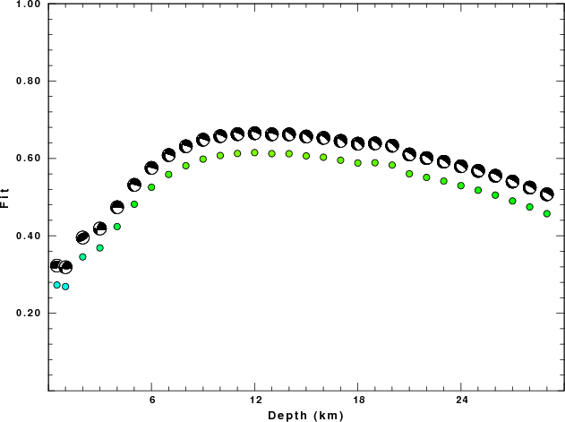
The best fit as a function of depth is given in the following figure:
|
|
|
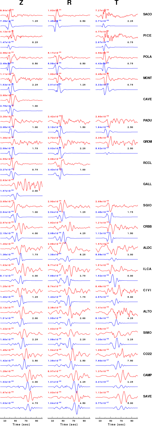
The comparison of the observed and predicted waveforms is given in the next figure. The red traces are the observed and the blue are the predicted. Each observed-predicted componnet is plotted to the same scale and peak amplitudes are indicated by the numbers to the left of each trace. The number in black at the rightr of each predicted traces it the time shift required for maximum correlation between the observed and predicted traces. This time shift is required because the synthetics are not computed at exactly the same distance as the observed and because the velocity model used in the predictions may not be perfect. A positive time shift indicates that the prediction is too fast and should be delayed to match the observed trace (shift to the right in this figure). A negative value indicates that the prediction is too slow. The bandpass filter used in the processing and for the display was
hp c 0.02 n 3
lp c 0.10 n 3
|
|
|
|
| Focal mechanism sensitivity at the preferred depth. The red color indicates a very good fit to thewavefroms. Each solution is plotted as a vector at a given value of strike and dip with the angle of the vector representing the rake angle, measured, with respect to the upward vertical (N) in the figure. |
The following figure shows the stations used in the grid search for the best focal mechanism to fit the surface-wave spectral amplitudes of the Love and Rayleigh waves.

|
|
|
The surface-wave determined focal mechanism is shown here.
 |
The P-wave first motion data for focal mechanism studies are as follow:
Sta Az(deg)    Dist(km)   First motion
SACO      338   15 iP_D
PICE      117   22 eP_+
POLA      169   24 iP_C
SX17       87   35 iP_C
MONT      290   38 eP_+
PIAG      187   42 iP_C
VENO       50   43 iP_C
CAVE      227   44 iP_C
PADU      155   47 eP_-
GROM      321   50 eP_-
RCCL      215   57 iP_C
TRIC      101   58 eP_+
GALL      128   75 eP_X
SGIO      179   75 eP_+
CRBB       60   81 eP_+
CRAC      114   93 eP_X
ALDC      136  117 eP_X
ILCA       95  122 iP_C
CIVI      143  124 eP_X
ALTO      153  129 eP_X
SIMO      162  141 eP_X
CO22      151  155 eP_X
CAMP      140  188 eP_+
SAVE      143  194 eP_+
Surface wave analysis was performed using codes from Computer Programs in Seismology, specifically the multiple filter analysis program do_mft and the surface-wave radiation pattern search program srfgrd96.
The velocity model used for the search is a modified Utah model .
Digital data were collected, instrument response removed and traces converted
to Z, R an T components. Multiple filter analysis was applied to the Z and T traces to obtain the Rayleigh- and Love-wave spectral amplitudes, respectively.
These were input to the search program which examined all depths between 1 and 25 km
and all possible mechanisms.

|
|
|

|
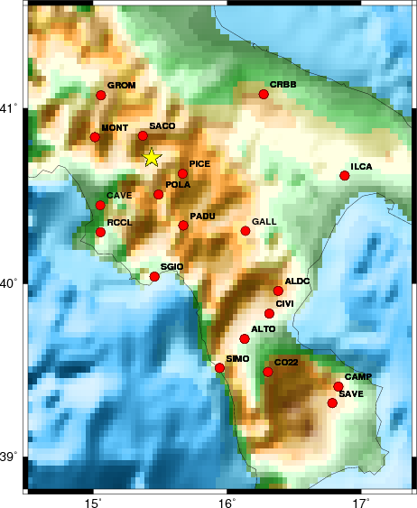
| Pressure-tension axis trends. Since the surface-wave spectra search does not distinguish between P and T axes and since there is a 180 ambiguity in strike, all possible P and T axes are plotted. First motion data and waveforms will be used to select the preferred mechanism. The purpose of this plot is to provide an idea of the possible range of solutions. The P and T-axes for all mechanisms with goodness of fit greater than 0.9 FITMAX (above) are plotted here. |

|
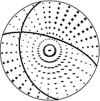
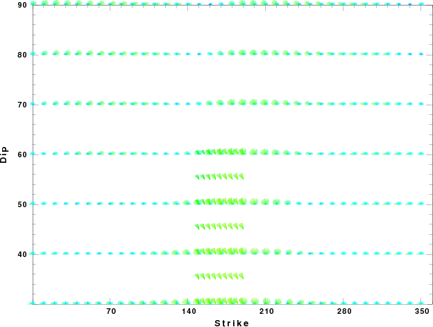
| Focal mechanism sensitivity at the preferred depth. The red color indicates a very good fit to the Love and Rayleigh wave radiation patterns. Each solution is plotted as a vector at a given value of strike and dip with the angle of the vector representing the rake angle, measured, with respect to the upward vertical (N) in the figure. Because of the symmetry of the spectral amplitude rediation patterns, only strikes from 0-180 degrees are sampled. |
Sta Az(deg) Dist(km)
Since the analysis of the surface-wave radiation patterns uses only spectral amplitudes and because the surfave-wave radiation patterns have a 180 degree symmetry, each surface-wave solution consists of four possible focal mechanisms corresponding to the interchange of the P- and T-axes and a roation of the mechanism by 180 degrees. To select one mechanism, P-wave first motion can be used. This was not possible in this case because all the P-wave first motions were emergent ( a feature of the P-wave wave takeoff angle, the station location and the mechanism). The other way to select among the mechanisms is to compute forward synthetics and compare the observed and predicted waveforms.
The velocity model used for the waveform fit is a modified Utah model .
The fits to the waveforms with the given mechanism are show below:

|
This figure shows the fit to the three components of motion (Z - vertical, R-radial and T - transverse). For each station and component, the observed traces is shown in red and the model predicted trace in blue. The traces represent filtered ground velocity in units of meters/sec (the peak value is printed adjacent to each trace; each pair of traces to plotted to the same scale to emphasize the difference in levels). Both synthetic and observed traces have been filtered using the SAC commands:

|

|
Should the national backbone of the USGS Advanced National Seismic System (ANSS) be implemented with an interstation separation of 300 km, it is very likely that an earthquake such as this would have been recorded at distances on the order of 100-200 km. This means that the closest station would have information on source depth and mechanism that was lacking here.
Dr. Harley Benz, USGS, provided the USGS USNSN digital data. The digital data used in this study were provided by Natural Resources Canada through their AUTODRM site http://www.seismo.nrcan.gc.ca/nwfa/autodrm/autodrm_req_e.php, and IRIS using their BUD interface
The figures below show the observed spectral amplitudes (units of cm-sec) at each station and the
theoretical predictions as a function of period for the mechanism given above. The modified Utah model earth model
was used to define the Green's functions. For each station, the Love and Rayleigh wave spectrail amplitudes are plotted with the same scaling so that one can get a sense fo the effects of the effects of the focal mechanism and depth on the excitation of each.
Here we tabulate the reasons for not using certain digital data sets
The following stations did not have a valid response files: