2014/04/15 17:12:19 -20.179 -70.781 15.8 4.7 Chile
USGS Felt map for this earthquake
 USGS/SLU Moment Tensor Solution
 ENS  2014/04/15 17:12:19:0 -20.18  -70.78  15.8 4.7 Chile

 Stations used:
   C.GO01 C.GO02 CX.MNMCX CX.PATCX CX.PB01 CX.PB04 CX.PB06
   CX.PB07 CX.PB08 CX.PB09 CX.PB10 CX.PB11 CX.PB12 CX.PB14
   CX.PB15 CX.PB16 CX.PSGCX GT.LPAZ IU.LVC

 Filtering commands used:
   cut a -30 a 180
   rtr
   taper w 0.1
   hp c 0.02 n 3
   lp c 0.06 n 3

 Best Fitting Double Couple
  Mo = 1.62e+23 dyne-cm
  Mw = 4.74
  Z  = 18 km
  Plane   Strike  Dip  Rake
   NP1      170    65    90
   NP2      350    25    90
  Principal Axes:
   Axis    Value   Plunge  Azimuth
    T   1.62e+23     70      80
    N   0.00e+00     -0     170
    P  -1.62e+23     20     260

 Moment Tensor: (dyne-cm)
    Component   Value
       Mxx    -3.75e+21
       Mxy    -2.12e+22
       Mxz     1.81e+22
       Myy    -1.20e+23
       Myz     1.03e+23
       Mzz     1.24e+23


                     ---######-----
                 ------###########-----
              --------##############------
             ---------################-----
           ----------###################-----
          -----------####################-----
         ------------#####################-----
        -------------######################-----
        -------------######################-----
       --------------###########   #########-----
       --------------########### T #########-----
       ---   ---------##########   #########-----
       --- P ---------######################-----
        --   ----------#####################----
        ---------------####################-----
         ---------------###################----
          --------------##################----
           --------------################----
             -------------##############---
              -------------###########----
                 ------------#######---
                     ---------####-


 Global CMT Convention Moment Tensor:
      R          T          P
  1.24e+23   1.81e+22  -1.03e+23
  1.81e+22  -3.75e+21   2.12e+22
 -1.03e+23   2.12e+22  -1.20e+23


Details of the solution is found at

http://www.eas.slu.edu/eqc/eqc_mt/MECH.NA/20140415171219/index.html
|
      STK = 170
      DIP = 65
     RAKE = 90
       MW = 4.74
       HS = 18.0
The NDK file is 20140415171219.ndk The waveform inversion is preferred.
The following compares this source inversion to others
 USGS/SLU Moment Tensor Solution
 ENS  2014/04/15 17:12:19:0 -20.18  -70.78  15.8 4.7 Chile

 Stations used:
   C.GO01 C.GO02 CX.MNMCX CX.PATCX CX.PB01 CX.PB04 CX.PB06
   CX.PB07 CX.PB08 CX.PB09 CX.PB10 CX.PB11 CX.PB12 CX.PB14
   CX.PB15 CX.PB16 CX.PSGCX GT.LPAZ IU.LVC

 Filtering commands used:
   cut a -30 a 180
   rtr
   taper w 0.1
   hp c 0.02 n 3
   lp c 0.06 n 3

 Best Fitting Double Couple
  Mo = 1.62e+23 dyne-cm
  Mw = 4.74
  Z  = 18 km
  Plane   Strike  Dip  Rake
   NP1      170    65    90
   NP2      350    25    90
  Principal Axes:
   Axis    Value   Plunge  Azimuth
    T   1.62e+23     70      80
    N   0.00e+00     -0     170
    P  -1.62e+23     20     260

 Moment Tensor: (dyne-cm)
    Component   Value
       Mxx    -3.75e+21
       Mxy    -2.12e+22
       Mxz     1.81e+22
       Myy    -1.20e+23
       Myz     1.03e+23
       Mzz     1.24e+23


                     ---######-----
                 ------###########-----
              --------##############------
             ---------################-----
           ----------###################-----
          -----------####################-----
         ------------#####################-----
        -------------######################-----
        -------------######################-----
       --------------###########   #########-----
       --------------########### T #########-----
       ---   ---------##########   #########-----
       --- P ---------######################-----
        --   ----------#####################----
        ---------------####################-----
         ---------------###################----
          --------------##################----
           --------------################----
             -------------##############---
              -------------###########----
                 ------------#######---
                     ---------####-


 Global CMT Convention Moment Tensor:
      R          T          P
  1.24e+23   1.81e+22  -1.03e+23
  1.81e+22  -3.75e+21   2.12e+22
 -1.03e+23   2.12e+22  -1.20e+23


Details of the solution is found at

http://www.eas.slu.edu/eqc/eqc_mt/MECH.NA/20140415171219/index.html
|
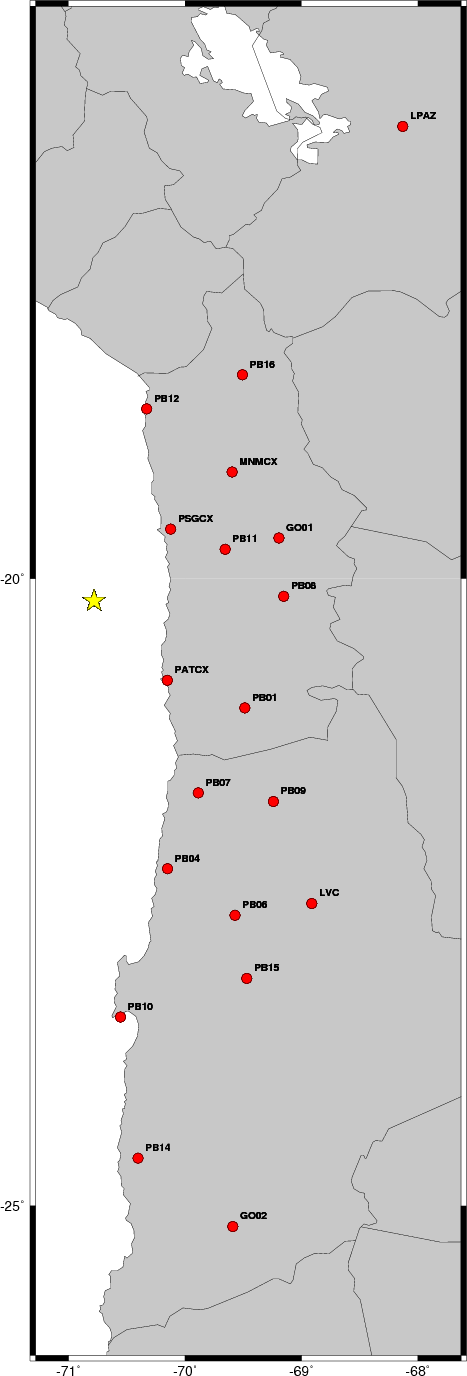
The focal mechanism was determined using broadband seismic waveforms. The location of the event and the and stations used for the waveform inversion are shown in the next figure.
|
|
|
|
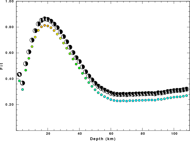
The program wvfgrd96 was used with good traces observed at short distance to determine the focal mechanism, depth and seismic moment. This technique requires a high quality signal and well determined velocity model for the Green functions. To the extent that these are the quality data, this type of mechanism should be preferred over the radiation pattern technique which requires the separate step of defining the pressure and tension quadrants and the correct strike.
The observed and predicted traces are filtered using the following gsac commands:
cut a -30 a 180
rtr
taper w 0.1
hp c 0.02 n 3
lp c 0.06 n 3
The results of this grid search from 0.5 to 19 km depth are as follow:
           DEPTH  STK   DIP  RAKE   MW    FIT
WVFGRD96    2.0   155    45   -90   4.47 0.3841
WVFGRD96    4.0   170    90    80   4.58 0.3172
WVFGRD96    6.0   350    90   -85   4.58 0.4667
WVFGRD96    8.0   170    85    85   4.66 0.5583
WVFGRD96   10.0   170    75    90   4.68 0.6492
WVFGRD96   12.0   170    70    90   4.70 0.7221
WVFGRD96   14.0   170    70    90   4.71 0.7745
WVFGRD96   16.0   170    65    90   4.73 0.8024
WVFGRD96   18.0   170    65    90   4.74 0.8131
WVFGRD96   20.0   170    65    90   4.74 0.8088
WVFGRD96   22.0   350    25    90   4.76 0.7955
WVFGRD96   24.0   355    25    95   4.77 0.7732
WVFGRD96   26.0   365    20   105   4.78 0.7457
WVFGRD96   28.0   170    70    85   4.78 0.7133
WVFGRD96   30.0   170    70    85   4.79 0.6765
WVFGRD96   32.0   170    70    85   4.79 0.6364
WVFGRD96   34.0   170    70    85   4.80 0.5944
WVFGRD96   36.0   170    70    85   4.80 0.5527
WVFGRD96   38.0   170    70    85   4.80 0.5136
WVFGRD96   40.0   170    80    85   4.94 0.4834
WVFGRD96   42.0   170    75    85   4.93 0.4423
WVFGRD96   44.0   370    15   110   4.93 0.4047
WVFGRD96   46.0   170    75    85   4.93 0.3712
WVFGRD96   48.0   170    70    85   4.93 0.3416
WVFGRD96   50.0   365    20   105   4.94 0.3152
WVFGRD96   52.0   145    60    60   4.94 0.2928
WVFGRD96   54.0   145    60    60   4.94 0.2766
WVFGRD96   56.0   150    60    65   4.94 0.2620
WVFGRD96   58.0   125    70    50   4.95 0.2501
WVFGRD96   60.0   130    70    50   4.94 0.2392
WVFGRD96   62.0   120    50    25   4.97 0.2327
WVFGRD96   64.0   125    50    35   4.97 0.2296
WVFGRD96   66.0   130    50    40   4.97 0.2286
WVFGRD96   68.0   130    50    40   4.98 0.2306
WVFGRD96   70.0   135    50    50   4.98 0.2278
WVFGRD96   72.0   135    50    50   4.99 0.2313
WVFGRD96   74.0   130    55    45   4.99 0.2303
WVFGRD96   76.0   135    55    50   5.00 0.2326
WVFGRD96   78.0   135    55    50   5.00 0.2332
WVFGRD96   80.0   140    55    60   5.01 0.2340
WVFGRD96   82.0   135    55    50   5.01 0.2346
WVFGRD96   84.0   140    55    55   5.01 0.2361
WVFGRD96   86.0   140    55    55   5.01 0.2360
WVFGRD96   88.0   140    55    55   5.01 0.2347
WVFGRD96   90.0   150    45    55   5.01 0.2413
WVFGRD96   92.0   150    50    60   5.01 0.2409
WVFGRD96   94.0   150    50    60   5.02 0.2453
WVFGRD96   96.0   155    50    65   5.02 0.2509
WVFGRD96   98.0   155    50    65   5.02 0.2536
WVFGRD96  100.0   155    50    65   5.03 0.2579
WVFGRD96  102.0   165    45    75   5.02 0.2601
WVFGRD96  104.0   165    45    75   5.02 0.2611
WVFGRD96  106.0   165    50    80   5.03 0.2654
WVFGRD96  108.0   165    50    80   5.03 0.2701
The best solution is
WVFGRD96 18.0 170 65 90 4.74 0.8131
The mechanism correspond to the best fit is
|
|
|
The best fit as a function of depth is given in the following figure:
|
|
|
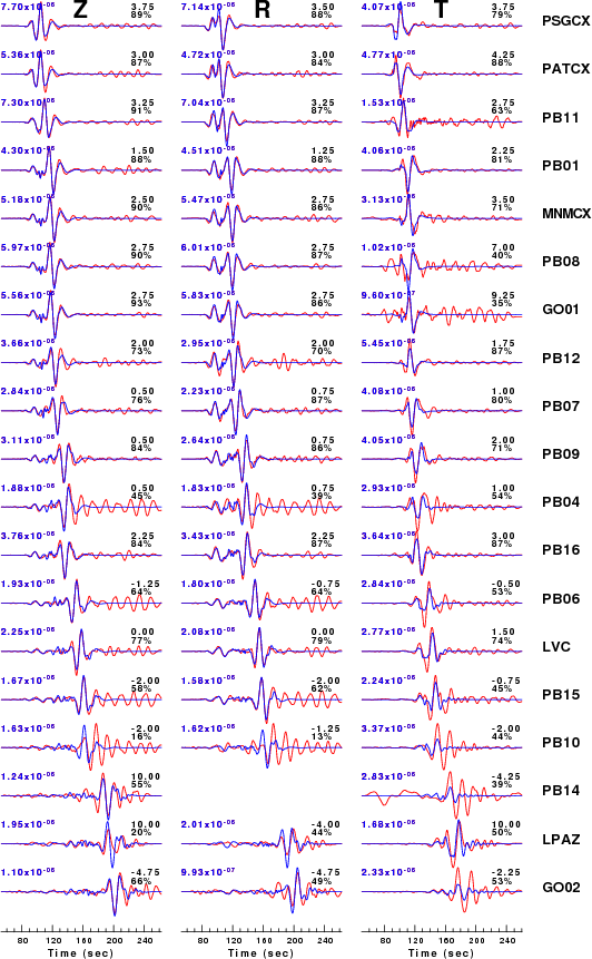
The comparison of the observed and predicted waveforms is given in the next figure. The red traces are the observed and the blue are the predicted. Each observed-predicted component is plotted to the same scale and peak amplitudes are indicated by the numbers to the left of each trace. A pair of numbers is given in black at the right of each predicted traces. The upper number it the time shift required for maximum correlation between the observed and predicted traces. This time shift is required because the synthetics are not computed at exactly the same distance as the observed and because the velocity model used in the predictions may not be perfect. A positive time shift indicates that the prediction is too fast and should be delayed to match the observed trace (shift to the right in this figure). A negative value indicates that the prediction is too slow. The lower number gives the percentage of variance reduction to characterize the individual goodness of fit (100% indicates a perfect fit).
The bandpass filter used in the processing and for the display was
cut a -30 a 180
rtr
taper w 0.1
hp c 0.02 n 3
lp c 0.06 n 3
|
|
|
|
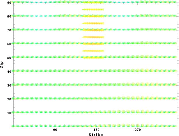
| Focal mechanism sensitivity at the preferred depth. The red color indicates a very good fit to thewavefroms. Each solution is plotted as a vector at a given value of strike and dip with the angle of the vector representing the rake angle, measured, with respect to the upward vertical (N) in the figure. |
A check on the assumed source location is possible by looking at the time shifts between the observed and predicted traces. The time shifts for waveform matching arise for several reasons:
Time_shift = A + B cos Azimuth + C Sin Azimuth
The time shifts for this inversion lead to the next figure:
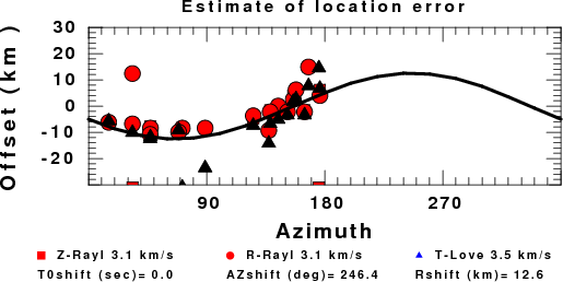
The derived shift in origin time and epicentral coordinates are given at the bottom of the figure.
Thanks also to the many seismic network operators whose dedication make this effort possible: University of Nevada Reno, University of Alaska, University of Washington, Oregon State University, University of Utah, Montana Bureas of Mines, UC Berkely, Caltech, UC San Diego, Saint Louis University, University of Memphis, Lamont Doherty Earth Observatory, the Iris stations and the Transportable Array of EarthScope.
The WUS used for the waveform synthetic seismograms and for the surface wave eigenfunctions and dispersion is as follows:
MODEL.01
Model after     8 iterations
ISOTROPIC
KGS
FLAT EARTH
1-D
CONSTANT VELOCITY
LINE08
LINE09
LINE10
LINE11
      H(KM)   VP(KM/S)   VS(KM/S) RHO(GM/CC)         QP         QS       ETAP       ETAS      FREFP      FREFS
     1.9000     3.4065     2.0089     2.2150  0.302E-02  0.679E-02   0.00       0.00       1.00       1.00
     6.1000     5.5445     3.2953     2.6089  0.349E-02  0.784E-02   0.00       0.00       1.00       1.00
    13.0000     6.2708     3.7396     2.7812  0.212E-02  0.476E-02   0.00       0.00       1.00       1.00
    19.0000     6.4075     3.7680     2.8223  0.111E-02  0.249E-02   0.00       0.00       1.00       1.00
     0.0000     7.9000     4.6200     3.2760  0.164E-10  0.370E-10   0.00       0.00       1.00       1.00
Here we tabulate the reasons for not using certain digital data sets
The following stations did not have a valid response files: