2014/04/15 16:21:16 -20.160 -70.754 10.4 5.5 Chile
USGS Felt map for this earthquake
 USGS/SLU Moment Tensor Solution
 ENS  2014/04/15 16:21:16:0 -20.16  -70.75  10.4 5.5 Chile

 Stations used:
   C.GO01 CX.MNMCX CX.PATCX CX.PB01 CX.PB04 CX.PB06 CX.PB07
   CX.PB08 CX.PB09 CX.PB10 CX.PB11 CX.PB12 CX.PB14 CX.PB15
   CX.PB16 CX.PSGCX GT.LPAZ IU.LVC

 Filtering commands used:
   cut a -30 a 180
   rtr
   taper w 0.1
   hp c 0.02 n 3
   lp c 0.06 n 3

 Best Fitting Double Couple
  Mo = 3.72e+23 dyne-cm
  Mw = 4.98
  Z  = 10 km
  Plane   Strike  Dip  Rake
   NP1       98    50   113
   NP2      245    45    65
  Principal Axes:
   Axis    Value   Plunge  Azimuth
    T   3.72e+23     72      74
    N   0.00e+00     17     263
    P  -3.72e+23      3     172

 Moment Tensor: (dyne-cm)
    Component   Value
       Mxx    -3.62e+23
       Mxy     5.76e+22
       Mxz     4.69e+22
       Myy     2.49e+22
       Myz     1.01e+23
       Mzz     3.37e+23


                     --------------
                 ----------------------
              ----------------------------
             ------------------------------
           -----------------############-----
          -------------######################-
         -----------###########################
        ---------###############################
        -------#################################
       #------################   ################
       ##---################## T ################
       ###-###################   ################
       ###-######################################
        ##----#################################-
        #-------#############################---
         -----------#####################------
          -------------------####-------------
           ----------------------------------
             ------------------------------
              ----------------------------
                 ------------   -------
                     -------- P ---


 Global CMT Convention Moment Tensor:
      R          T          P
  3.37e+23   4.69e+22  -1.01e+23
  4.69e+22  -3.62e+23  -5.76e+22
 -1.01e+23  -5.76e+22   2.49e+22


Details of the solution is found at

http://www.eas.slu.edu/eqc/eqc_mt/MECH.NA/20140415162116/index.html
|
      STK = 245
      DIP = 45
     RAKE = 65
       MW = 4.98
       HS = 10.0
The NDK file is 20140415162116.ndk The waveform inversion is preferred.
The following compares this source inversion to others
 USGS/SLU Moment Tensor Solution
 ENS  2014/04/15 16:21:16:0 -20.16  -70.75  10.4 5.5 Chile

 Stations used:
   C.GO01 CX.MNMCX CX.PATCX CX.PB01 CX.PB04 CX.PB06 CX.PB07
   CX.PB08 CX.PB09 CX.PB10 CX.PB11 CX.PB12 CX.PB14 CX.PB15
   CX.PB16 CX.PSGCX GT.LPAZ IU.LVC

 Filtering commands used:
   cut a -30 a 180
   rtr
   taper w 0.1
   hp c 0.02 n 3
   lp c 0.06 n 3

 Best Fitting Double Couple
  Mo = 3.72e+23 dyne-cm
  Mw = 4.98
  Z  = 10 km
  Plane   Strike  Dip  Rake
   NP1       98    50   113
   NP2      245    45    65
  Principal Axes:
   Axis    Value   Plunge  Azimuth
    T   3.72e+23     72      74
    N   0.00e+00     17     263
    P  -3.72e+23      3     172

 Moment Tensor: (dyne-cm)
    Component   Value
       Mxx    -3.62e+23
       Mxy     5.76e+22
       Mxz     4.69e+22
       Myy     2.49e+22
       Myz     1.01e+23
       Mzz     3.37e+23


                     --------------
                 ----------------------
              ----------------------------
             ------------------------------
           -----------------############-----
          -------------######################-
         -----------###########################
        ---------###############################
        -------#################################
       #------################   ################
       ##---################## T ################
       ###-###################   ################
       ###-######################################
        ##----#################################-
        #-------#############################---
         -----------#####################------
          -------------------####-------------
           ----------------------------------
             ------------------------------
              ----------------------------
                 ------------   -------
                     -------- P ---


 Global CMT Convention Moment Tensor:
      R          T          P
  3.37e+23   4.69e+22  -1.01e+23
  4.69e+22  -3.62e+23  -5.76e+22
 -1.01e+23  -5.76e+22   2.49e+22


Details of the solution is found at

http://www.eas.slu.edu/eqc/eqc_mt/MECH.NA/20140415162116/index.html
|
April 15, 2014, NEAR COAST OF NORTHERN CHILE, MW=5.1

Howard Koss

CENTROID-MOMENT-TENSOR  SOLUTION
GCMT EVENT:     C201404151621A
DATA: II DK IU MN G  CU LD GE KP
 IC
L.P.BODY WAVES: 71S,  83C, T= 40
SURFACE WAVES: 115S, 173C, T= 50
TIMESTAMP:      Q-20140415144455
CENTROID LOCATION:
ORIGIN TIME:      16:21:22.0 0.2
LAT:20.21S 0.01;LON: 70.70W 0.02
DEP: 12.7  0.6;TRIANG HDUR:  0.9
MOMENT TENSOR: SCALE 10**23 D-CM
RR= 5.460 0.206; TT=-5.300 0.139
PP=-0.166 0.168; RT=-1.940 0.336
RP= 3.150 0.601; TP=-0.194 0.119
PRINCIPAL AXES:
1.(T) VAL=  7.146;PLG=65;AZM=250
2.(N)      -1.486;    22;     99
3.(P)      -5.666;    11;      4
BEST DBLE.COUPLE:M0= 6.41*10**23
NP1: STRIKE= 69;DIP=39;SLIP=  53
NP2: STRIKE=293;DIP=60;SLIP= 116

            ----- P ---
        ---------   -------
      -----------------------
    ---------------------------
   -----------------------------
  ################---------------
  ####################-----------
 ########################-------##
 ##########   ##############----##
 ########## T ###############--###
 ##########   ################-###
  ##########################----#
  -#######################-------
   --###################--------
    -----##########------------
      -----------------------
        -------------------
            -----------
|
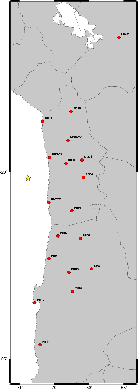
The focal mechanism was determined using broadband seismic waveforms. The location of the event and the and stations used for the waveform inversion are shown in the next figure.
|
|
|
|
The program wvfgrd96 was used with good traces observed at short distance to determine the focal mechanism, depth and seismic moment. This technique requires a high quality signal and well determined velocity model for the Green functions. To the extent that these are the quality data, this type of mechanism should be preferred over the radiation pattern technique which requires the separate step of defining the pressure and tension quadrants and the correct strike.
The observed and predicted traces are filtered using the following gsac commands:
cut a -30 a 180
rtr
taper w 0.1
hp c 0.02 n 3
lp c 0.06 n 3
The results of this grid search from 0.5 to 19 km depth are as follow:
           DEPTH  STK   DIP  RAKE   MW    FIT
WVFGRD96    2.0    30    85    10   4.65 0.4040
WVFGRD96    4.0   220    40    15   4.80 0.4568
WVFGRD96    6.0   230    50    40   4.84 0.5486
WVFGRD96    8.0   240    45    60   4.95 0.6431
WVFGRD96   10.0   245    45    65   4.98 0.7032
WVFGRD96   12.0   245    45    65   4.98 0.6853
WVFGRD96   14.0   225    55    35   4.95 0.6467
WVFGRD96   16.0   225    60    30   4.95 0.6067
WVFGRD96   18.0   225    60    30   4.95 0.5700
WVFGRD96   20.0   220    65    20   4.96 0.5356
WVFGRD96   22.0   220    65    20   4.97 0.5050
WVFGRD96   24.0   220    65    20   4.98 0.4747
WVFGRD96   26.0   220    65    15   4.99 0.4478
WVFGRD96   28.0   220    65    15   5.00 0.4227
WVFGRD96   30.0   220    70    15   5.01 0.3999
WVFGRD96   32.0   220    70    15   5.02 0.3785
WVFGRD96   34.0   220    70    15   5.03 0.3588
WVFGRD96   36.0   220    75    15   5.04 0.3417
WVFGRD96   38.0   220    75    15   5.06 0.3289
WVFGRD96   40.0   215    80    20   5.12 0.3207
WVFGRD96   42.0   215    80    15   5.13 0.3135
WVFGRD96   44.0   215    80    15   5.14 0.3056
WVFGRD96   46.0   215    80    15   5.15 0.2977
WVFGRD96   48.0   215    80    15   5.16 0.2907
WVFGRD96   50.0   215    85    20   5.17 0.2842
WVFGRD96   52.0   215    80    15   5.18 0.2789
WVFGRD96   54.0   120    90   -20   5.20 0.2717
WVFGRD96   56.0   120    90   -20   5.21 0.2729
WVFGRD96   58.0   120    90   -20   5.22 0.2715
WVFGRD96   60.0   300    90    20   5.23 0.2731
WVFGRD96   62.0   120    90   -15   5.23 0.2741
WVFGRD96   64.0   120    90   -15   5.24 0.2728
WVFGRD96   66.0   120    80   -20   5.25 0.2689
WVFGRD96   68.0   120    80   -15   5.26 0.2702
WVFGRD96   70.0   120    80   -15   5.26 0.2708
WVFGRD96   72.0   120    80   -15   5.27 0.2724
WVFGRD96   74.0   210    80     5   5.27 0.2702
WVFGRD96   76.0   210    80     0   5.26 0.2718
WVFGRD96   78.0    35    70   -30   5.27 0.2769
WVFGRD96   80.0    35    65   -35   5.28 0.2792
WVFGRD96   82.0    35    60   -35   5.28 0.2829
WVFGRD96   84.0    35    60   -35   5.28 0.2865
WVFGRD96   86.0    20    40   -60   5.29 0.2886
WVFGRD96   88.0    25    40   -55   5.29 0.2929
WVFGRD96   90.0    25    40   -55   5.30 0.2962
WVFGRD96   92.0    20    35   -60   5.31 0.2997
WVFGRD96   94.0    20    35   -60   5.31 0.3028
WVFGRD96   96.0    20    35   -60   5.31 0.3060
WVFGRD96   98.0    25    35   -55   5.31 0.3087
WVFGRD96  100.0    25    35   -55   5.32 0.3120
WVFGRD96  102.0    20    30   -60   5.32 0.3144
WVFGRD96  104.0    20    30   -60   5.33 0.3174
WVFGRD96  106.0    20    30   -60   5.33 0.3197
WVFGRD96  108.0    20    30   -60   5.33 0.3226
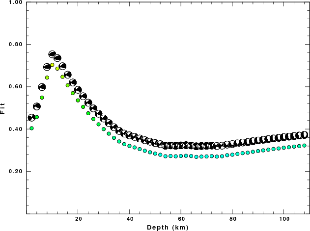
The best solution is
WVFGRD96 10.0 245 45 65 4.98 0.7032
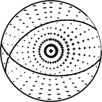
The mechanism correspond to the best fit is
|
|
|
The best fit as a function of depth is given in the following figure:
|
|
|
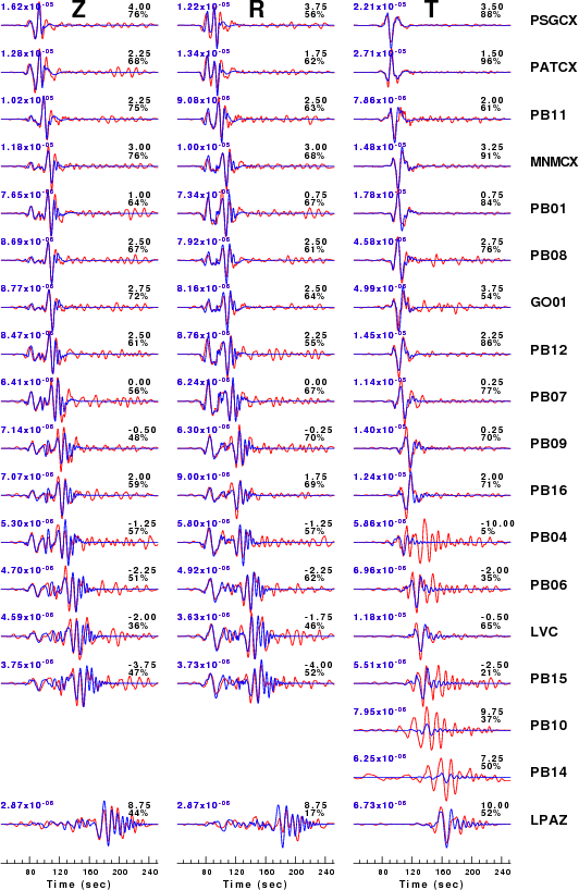
The comparison of the observed and predicted waveforms is given in the next figure. The red traces are the observed and the blue are the predicted. Each observed-predicted component is plotted to the same scale and peak amplitudes are indicated by the numbers to the left of each trace. A pair of numbers is given in black at the right of each predicted traces. The upper number it the time shift required for maximum correlation between the observed and predicted traces. This time shift is required because the synthetics are not computed at exactly the same distance as the observed and because the velocity model used in the predictions may not be perfect. A positive time shift indicates that the prediction is too fast and should be delayed to match the observed trace (shift to the right in this figure). A negative value indicates that the prediction is too slow. The lower number gives the percentage of variance reduction to characterize the individual goodness of fit (100% indicates a perfect fit).
The bandpass filter used in the processing and for the display was
cut a -30 a 180
rtr
taper w 0.1
hp c 0.02 n 3
lp c 0.06 n 3
|
|
|
|
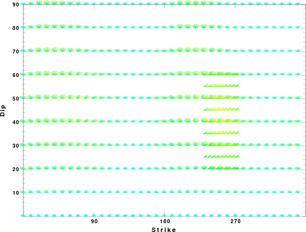
| Focal mechanism sensitivity at the preferred depth. The red color indicates a very good fit to thewavefroms. Each solution is plotted as a vector at a given value of strike and dip with the angle of the vector representing the rake angle, measured, with respect to the upward vertical (N) in the figure. |
A check on the assumed source location is possible by looking at the time shifts between the observed and predicted traces. The time shifts for waveform matching arise for several reasons:
Time_shift = A + B cos Azimuth + C Sin Azimuth
The time shifts for this inversion lead to the next figure:
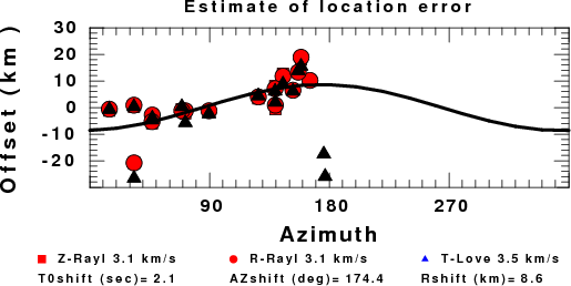
The derived shift in origin time and epicentral coordinates are given at the bottom of the figure.
Thanks also to the many seismic network operators whose dedication make this effort possible: University of Nevada Reno, University of Alaska, University of Washington, Oregon State University, University of Utah, Montana Bureas of Mines, UC Berkely, Caltech, UC San Diego, Saint Louis University, University of Memphis, Lamont Doherty Earth Observatory, the Iris stations and the Transportable Array of EarthScope.
The WUS used for the waveform synthetic seismograms and for the surface wave eigenfunctions and dispersion is as follows:
MODEL.01
Model after     8 iterations
ISOTROPIC
KGS
FLAT EARTH
1-D
CONSTANT VELOCITY
LINE08
LINE09
LINE10
LINE11
      H(KM)   VP(KM/S)   VS(KM/S) RHO(GM/CC)         QP         QS       ETAP       ETAS      FREFP      FREFS
     1.9000     3.4065     2.0089     2.2150  0.302E-02  0.679E-02   0.00       0.00       1.00       1.00
     6.1000     5.5445     3.2953     2.6089  0.349E-02  0.784E-02   0.00       0.00       1.00       1.00
    13.0000     6.2708     3.7396     2.7812  0.212E-02  0.476E-02   0.00       0.00       1.00       1.00
    19.0000     6.4075     3.7680     2.8223  0.111E-02  0.249E-02   0.00       0.00       1.00       1.00
     0.0000     7.9000     4.6200     3.2760  0.164E-10  0.370E-10   0.00       0.00       1.00       1.00
Here we tabulate the reasons for not using certain digital data sets
The following stations did not have a valid response files: