Location

2014/04/13 12:11:30 -20.621 -70.715 18.6 5.3 Chile

Arrival Times (from USGS)

Arrival time list

Felt Map

USGS Felt map for this earthquake

USGS Felt reports main page

Focal Mechanism

USGS/SLU Moment Tensor Solution ENS 2014/04/13 12:11:30:0 -20.62 -70.71 18.6 5.3 Chile Stations used: C.GO01 C.GO02 CX.MNMCX CX.PATCX CX.PB01 CX.PB04 CX.PB06 CX.PB07 CX.PB08 CX.PB09 CX.PB10 CX.PB11 CX.PB12 CX.PB14 CX.PB15 CX.PB16 CX.PSGCX GT.LPAZ IU.LVC Filtering commands used: cut a -30 a 180 rtr taper w 0.1 hp c 0.02 n 3 lp c 0.06 n 3 Best Fitting Double Couple Mo = 1.01e+24 dyne-cm Mw = 5.27 Z = 20 km Plane Strike Dip Rake NP1 160 75 85 NP2 359 16 108 Principal Axes: Axis Value Plunge Azimuth T 1.01e+24 60 63 N 0.00e+00 5 161 P -1.01e+24 30 254 Moment Tensor: (dyne-cm) Component Value Mxx -4.20e+21 Mxy -9.67e+22 Mxz 3.20e+23 Myy -5.00e+23 Myz 8.12e+23 Mzz 5.04e+23 ############-- ----###############--- -------##################--- --------####################-- ----------#####################--- -----------######################--- -------------######################--- --------------#######################--- ---------------######### ##########--- ----------------######### T ###########--- -----------------######## ###########--- -----------------######################--- ----- ----------#####################--- ---- P -----------###################--- ---- -----------###################--- ------------------#################--- ------------------###############--- ------------------#############--- -----------------###########-- ------------------#######--- ----------------###--- ------------## Global CMT Convention Moment Tensor: R T P 5.04e+23 3.20e+23 -8.12e+23 3.20e+23 -4.20e+21 9.67e+22 -8.12e+23 9.67e+22 -5.00e+23 Details of the solution is found at http://www.eas.slu.edu/eqc/eqc_mt/MECH.NA/20140413121130/index.html

Preferred Solution

      STK = 160
      DIP = 75
     RAKE = 85
       MW = 5.27
       HS = 20.0

The NDK file is 20140413121130.ndk The waveform inversion is preferred.

Moment Tensor Comparison

The following compares this source inversion to others

SLU	USGSMT
USGS/SLU Moment Tensor Solution ENS 2014/04/13 12:11:30:0 -20.62 -70.71 18.6 5.3 Chile Stations used: C.GO01 C.GO02 CX.MNMCX CX.PATCX CX.PB01 CX.PB04 CX.PB06 CX.PB07 CX.PB08 CX.PB09 CX.PB10 CX.PB11 CX.PB12 CX.PB14 CX.PB15 CX.PB16 CX.PSGCX GT.LPAZ IU.LVC Filtering commands used: cut a -30 a 180 rtr taper w 0.1 hp c 0.02 n 3 lp c 0.06 n 3 Best Fitting Double Couple Mo = 1.01e+24 dyne-cm Mw = 5.27 Z = 20 km Plane Strike Dip Rake NP1 160 75 85 NP2 359 16 108 Principal Axes: Axis Value Plunge Azimuth T 1.01e+24 60 63 N 0.00e+00 5 161 P -1.01e+24 30 254 Moment Tensor: (dyne-cm) Component Value Mxx -4.20e+21 Mxy -9.67e+22 Mxz 3.20e+23 Myy -5.00e+23 Myz 8.12e+23 Mzz 5.04e+23 ############-- ----###############--- -------##################--- --------####################-- ----------#####################--- -----------######################--- -------------######################--- --------------#######################--- ---------------######### ##########--- ----------------######### T ###########--- -----------------######## ###########--- -----------------######################--- ----- ----------#####################--- ---- P -----------###################--- ---- -----------###################--- ------------------#################--- ------------------###############--- ------------------#############--- -----------------###########-- ------------------#######--- ----------------###--- ------------## Global CMT Convention Moment Tensor: R T P 5.04e+23 3.20e+23 -8.12e+23 3.20e+23 -4.20e+21 9.67e+22 -8.12e+23 9.67e+22 -5.00e+23 Details of the solution is found at http://www.eas.slu.edu/eqc/eqc_mt/MECH.NA/20140413121130/index.html	Regional Moment Tensor (Mwr) Moment magnitude derived from a moment tensor inversion of complete waveforms at regional distances (less than ~8 degrees), generally used for the analysis of small to moderate size earthquakes (typically Mw 3.5-6.0) crust or upper mantle earthquakes. Moment 1.12e+17 N-m Magnitude 5.3 Percent DC 80% Depth 15.0 km Updated 2014-04-13 12:38:26 UTC Author us Catalog us Contributor us Code us_c000pipx_mwr Principal Axes Axis Value Plunge Azimuth T 1.060 55 60 N 0.104 7 160 P -1.164 34 255 Nodal Planes Plane Strike Dip Rake NP1 159 79 83 NP2 13 13 123

Waveform Inversion

The focal mechanism was determined using broadband seismic waveforms. The location of the event and the and stations used for the waveform inversion are shown in the next figure.

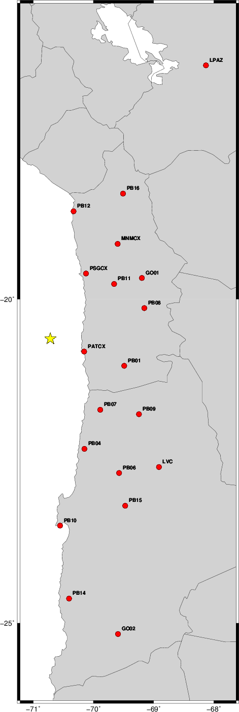
Location of broadband stations used for waveform inversion

The program wvfgrd96 was used with good traces observed at short distance to determine the focal mechanism, depth and seismic moment. This technique requires a high quality signal and well determined velocity model for the Green functions. To the extent that these are the quality data, this type of mechanism should be preferred over the radiation pattern technique which requires the separate step of defining the pressure and tension quadrants and the correct strike.

The observed and predicted traces are filtered using the following gsac commands:

cut a -30 a 180
rtr
taper w 0.1
hp c 0.02 n 3 
lp c 0.06 n 3 

           DEPTH  STK   DIP  RAKE   MW    FIT
WVFGRD96    2.0   155    40    90   5.01 0.4057
WVFGRD96    4.0   160    85    85   5.12 0.3340
WVFGRD96    6.0   340    90   -85   5.12 0.5033
WVFGRD96    8.0   160    85    85   5.20 0.6062
WVFGRD96   10.0   160    85    85   5.21 0.7012
WVFGRD96   12.0   160    80    85   5.22 0.7678
WVFGRD96   14.0   160    80    85   5.24 0.8107
WVFGRD96   16.0   160    75    85   5.25 0.8374
WVFGRD96   18.0   160    75    85   5.26 0.8490
WVFGRD96   20.0   160    75    85   5.27 0.8493
WVFGRD96   22.0   160    75    90   5.30 0.8416
WVFGRD96   24.0   360    15   110   5.30 0.8270
WVFGRD96   26.0   345    10    95   5.32 0.8073
WVFGRD96   28.0   330    10    80   5.33 0.7830
WVFGRD96   30.0   325    10    75   5.34 0.7542
WVFGRD96   32.0   325    10    75   5.35 0.7215
WVFGRD96   34.0   330    10    80   5.35 0.6861
WVFGRD96   36.0   330    10    80   5.35 0.6508
WVFGRD96   38.0   160    80    90   5.35 0.6172
WVFGRD96   40.0   340     5    90   5.50 0.5890
WVFGRD96   42.0   340     5    90   5.50 0.5472
WVFGRD96   44.0   320    10    65   5.50 0.5073
WVFGRD96   46.0   320    10    65   5.50 0.4697
WVFGRD96   48.0   310    10    55   5.50 0.4341
WVFGRD96   50.0   310    10    55   5.50 0.4006
WVFGRD96   52.0   305    10    50   5.51 0.3695
WVFGRD96   54.0   295    10    40   5.51 0.3414
WVFGRD96   56.0   165    70    65   5.51 0.3200
WVFGRD96   58.0   165    70    65   5.52 0.3047
WVFGRD96   60.0   335    60    85   5.51 0.2960
WVFGRD96   62.0   335    60    80   5.52 0.2930
WVFGRD96   64.0   335    60    80   5.52 0.2880
WVFGRD96   66.0   175    35   105   5.53 0.2909
WVFGRD96   68.0   165    35    90   5.52 0.2898
WVFGRD96   70.0   165    35    90   5.53 0.2881
WVFGRD96   72.0   165    35    90   5.53 0.2899
WVFGRD96   74.0   165    35    90   5.54 0.2887
WVFGRD96   76.0   165    35    90   5.54 0.2873
WVFGRD96   78.0   170    40    95   5.55 0.2908
WVFGRD96   80.0   165    40    90   5.55 0.2930
WVFGRD96   82.0   345    50    90   5.55 0.2910
WVFGRD96   84.0   165    40    85   5.55 0.2919
WVFGRD96   86.0   165    40    85   5.55 0.2934
WVFGRD96   88.0   280    50   -80   5.56 0.2927
WVFGRD96   90.0   280    50   -80   5.56 0.2957
WVFGRD96   92.0   290    55   -80   5.57 0.2993
WVFGRD96   94.0   290    55   -80   5.57 0.3047
WVFGRD96   96.0   290    55   -80   5.57 0.3097
WVFGRD96   98.0   290    55   -80   5.58 0.3125
WVFGRD96  100.0   285    55   -85   5.59 0.3164
WVFGRD96  102.0   285    55   -85   5.59 0.3190
WVFGRD96  104.0   285    55   -85   5.59 0.3226
WVFGRD96  106.0   340    50   -90   5.60 0.3226
WVFGRD96  108.0   165    40   -85   5.60 0.3247

The best solution is

WVFGRD96   20.0   160    75    85   5.27 0.8493

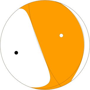
The mechanism correspond to the best fit is

Figure 1. Waveform inversion focal mechanism

The best fit as a function of depth is given in the following figure:

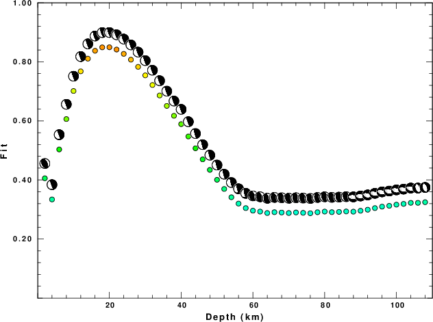
Figure 2. Depth sensitivity for waveform mechanism

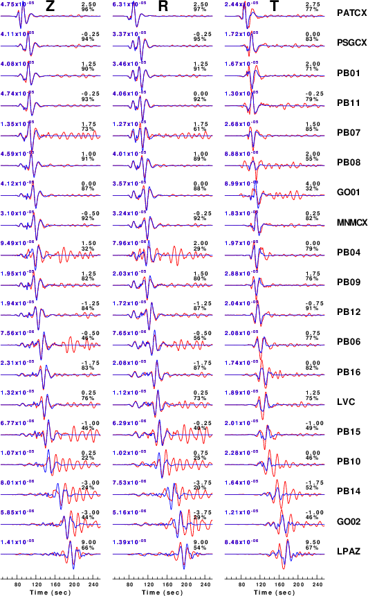
The comparison of the observed and predicted waveforms is given in the next figure. The red traces are the observed and the blue are the predicted. Each observed-predicted component is plotted to the same scale and peak amplitudes are indicated by the numbers to the left of each trace. A pair of numbers is given in black at the right of each predicted traces. The upper number it the time shift required for maximum correlation between the observed and predicted traces. This time shift is required because the synthetics are not computed at exactly the same distance as the observed and because the velocity model used in the predictions may not be perfect. A positive time shift indicates that the prediction is too fast and should be delayed to match the observed trace (shift to the right in this figure). A negative value indicates that the prediction is too slow. The lower number gives the percentage of variance reduction to characterize the individual goodness of fit (100% indicates a perfect fit).

The bandpass filter used in the processing and for the display was

cut a -30 a 180
rtr
taper w 0.1
hp c 0.02 n 3 
lp c 0.06 n 3 

Figure 3. Waveform comparison for selected depth. Red: observed; Blue - predicted. The time shift with respect to the model prediction is indicated. The percent of fit is also indicated.

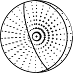
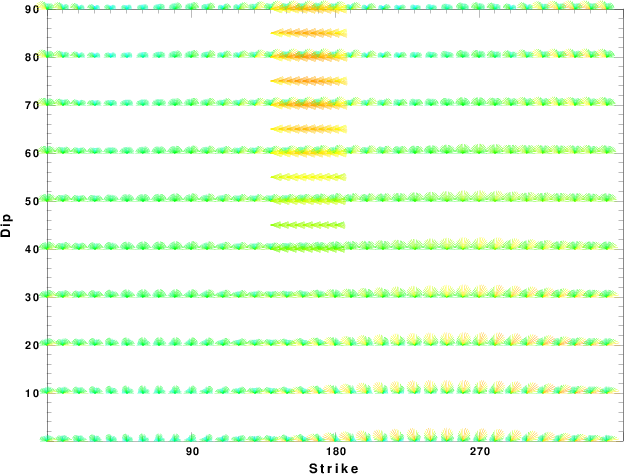
Focal mechanism sensitivity at the preferred depth. The red color indicates a very good fit to thewavefroms. Each solution is plotted as a vector at a given value of strike and dip with the angle of the vector representing the rake angle, measured, with respect to the upward vertical (N) in the figure.

A check on the assumed source location is possible by looking at the time shifts between the observed and predicted traces. The time shifts for waveform matching arise for several reasons:

• The origin time and epicentral distance are incorrect
• The velocity model used for the inversion is incorrect
• The velocity model used to define the P-arrival time is not the same as the velocity model used for the waveform inversion (assuming that the initial trace alignment is based on the P arrival time)

 Time_shift = A + B cos Azimuth + C Sin Azimuth

The time shifts for this inversion lead to the next figure:

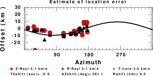
The derived shift in origin time and epicentral coordinates are given at the bottom of the figure.

Discussion

Acknowledgements

Thanks also to the many seismic network operators whose dedication make this effort possible: University of Nevada Reno, University of Alaska, University of Washington, Oregon State University, University of Utah, Montana Bureas of Mines, UC Berkely, Caltech, UC San Diego, Saint Louis University, University of Memphis, Lamont Doherty Earth Observatory, the Iris stations and the Transportable Array of EarthScope.

Velocity Model

The WUS used for the waveform synthetic seismograms and for the surface wave eigenfunctions and dispersion is as follows:

MODEL.01
Model after     8 iterations
ISOTROPIC
KGS
FLAT EARTH
1-D
CONSTANT VELOCITY
LINE08
LINE09
LINE10
LINE11
      H(KM)   VP(KM/S)   VS(KM/S) RHO(GM/CC)         QP         QS       ETAP       ETAS      FREFP      FREFS
     1.9000     3.4065     2.0089     2.2150  0.302E-02  0.679E-02   0.00       0.00       1.00       1.00    
     6.1000     5.5445     3.2953     2.6089  0.349E-02  0.784E-02   0.00       0.00       1.00       1.00    
    13.0000     6.2708     3.7396     2.7812  0.212E-02  0.476E-02   0.00       0.00       1.00       1.00    
    19.0000     6.4075     3.7680     2.8223  0.111E-02  0.249E-02   0.00       0.00       1.00       1.00    
     0.0000     7.9000     4.6200     3.2760  0.164E-10  0.370E-10   0.00       0.00       1.00       1.00    

Quality Control

Here we tabulate the reasons for not using certain digital data sets

The following stations did not have a valid response files: