Location
2014/04/11 00:01:44 -20.748 -70.724 17.5 6.0 Chile
Arrival Times (from USGS)
Arrival time list
Felt Map
USGS Felt map for this earthquake
USGS Felt reports main page
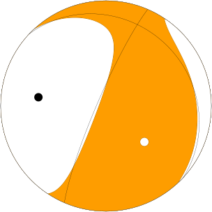
Focal Mechanism
 USGS/SLU Moment Tensor Solution
 ENS  2014/04/11 00:01:44:0 -20.75  -70.72  17.5 6.0 Chile

 Stations used:
   C.GO01 C.GO02 CX.MNMCX CX.PATCX CX.PB01 CX.PB04 CX.PB06
   CX.PB07 CX.PB08 CX.PB09 CX.PB10 CX.PB11 CX.PB12 CX.PB14
   CX.PB15 CX.PB16 CX.PSGCX GT.LPAZ

 Filtering commands used:
   cut a -30 a 180
   rtr
   taper w 0.1
   hp c 0.02 n 3
   lp c 0.06 n 3

 Best Fitting Double Couple
  Mo = 1.17e+25 dyne-cm
  Mw = 5.98
  Z  = 20 km
  Plane   Strike  Dip  Rake
   NP1      198    76   111
   NP2      320    25    35
  Principal Axes:
   Axis    Value   Plunge  Azimuth
    T   1.17e+25     54     133
    N   0.00e+00     20      12
    P  -1.17e+25     28     271

 Moment Tensor: (dyne-cm)
    Component   Value
       Mxx     1.87e+24
       Mxy    -1.84e+24
       Mxz    -3.90e+24
       Myy    -7.03e+24
       Myz     8.92e+24
       Mzz     5.16e+24


                     #############-
                 ##---------####-------
              -----------------##---------
             -----------------######-------
           ------------------#########-------
          ------------------############------
         ------------------##############------
        -------------------################-----
        ------------------#################-----
       ----   -----------###################-----
       ---- P -----------####################----
       ----   ----------#####################----
       ----------------######################----
        ---------------##########   #########---
        ---------------########## T #########---
         -------------###########   #########--
          ------------######################--
           -----------######################-
             ---------#####################
              -------####################-
                 ----##################
                     -#############


 Global CMT Convention Moment Tensor:
      R          T          P
  5.16e+24  -3.90e+24  -8.92e+24
 -3.90e+24   1.87e+24   1.84e+24
 -8.92e+24   1.84e+24  -7.03e+24


Details of the solution is found at

http://www.eas.slu.edu/eqc/eqc_mt/MECH.NA/20140411000144/index.html
|
Preferred Solution
The preferred solution from an analysis of the surface-wave spectral amplitude radiation pattern, waveform inversion and first motion observations is
      STK = 320
      DIP = 25
     RAKE = 35
       MW = 5.98
       HS = 20.0
The NDK file is 20140411000144.ndk
The waveform inversion is preferred.
Moment Tensor Comparison
The following compares this source inversion to others
| SLU |
USGSMT |
|
GCMT |
USGSW |
|
 USGS/SLU Moment Tensor Solution
 ENS  2014/04/11 00:01:44:0 -20.75  -70.72  17.5 6.0 Chile

 Stations used:
   C.GO01 C.GO02 CX.MNMCX CX.PATCX CX.PB01 CX.PB04 CX.PB06
   CX.PB07 CX.PB08 CX.PB09 CX.PB10 CX.PB11 CX.PB12 CX.PB14
   CX.PB15 CX.PB16 CX.PSGCX GT.LPAZ

 Filtering commands used:
   cut a -30 a 180
   rtr
   taper w 0.1
   hp c 0.02 n 3
   lp c 0.06 n 3

 Best Fitting Double Couple
  Mo = 1.17e+25 dyne-cm
  Mw = 5.98
  Z  = 20 km
  Plane   Strike  Dip  Rake
   NP1      198    76   111
   NP2      320    25    35
  Principal Axes:
   Axis    Value   Plunge  Azimuth
    T   1.17e+25     54     133
    N   0.00e+00     20      12
    P  -1.17e+25     28     271

 Moment Tensor: (dyne-cm)
    Component   Value
       Mxx     1.87e+24
       Mxy    -1.84e+24
       Mxz    -3.90e+24
       Myy    -7.03e+24
       Myz     8.92e+24
       Mzz     5.16e+24


                     #############-
                 ##---------####-------
              -----------------##---------
             -----------------######-------
           ------------------#########-------
          ------------------############------
         ------------------##############------
        -------------------################-----
        ------------------#################-----
       ----   -----------###################-----
       ---- P -----------####################----
       ----   ----------#####################----
       ----------------######################----
        ---------------##########   #########---
        ---------------########## T #########---
         -------------###########   #########--
          ------------######################--
           -----------######################-
             ---------#####################
              -------####################-
                 ----##################
                     -#############


 Global CMT Convention Moment Tensor:
      R          T          P
  5.16e+24  -3.90e+24  -8.92e+24
 -3.90e+24   1.87e+24   1.84e+24
 -8.92e+24   1.84e+24  -7.03e+24


Details of the solution is found at

http://www.eas.slu.edu/eqc/eqc_mt/MECH.NA/20140411000144/index.html
|
Regional Moment Tensor (Mwr)

Moment magnitude derived from a moment tensor
inversion of complete waveforms at regional
distances (less than ~8 degrees), generally
used for the analysis of small to moderate
size earthquakes (typically Mw 3.5-6.0)
crust or upper mantle earthquakes.

Moment
    1.25e+18 N-m
Magnitude
    6.0
Percent DC
    67%
Depth
    15.0 km
Updated
    2014-04-11 00:30:23 UTC
Author
    us
Catalog
    us
Contributor
    us
Code
    us_c000pfgr_mwr

Principal Axes
Axis	Value	Plunge	Azimuth
T	1.147	49 	133
N	0.186	18 	21
P	-1.333	36 	277
Nodal Planes
Plane	Strike	Dip	Rake
NP1	203°	83 	108
NP2	313°	20 	21
|
|
April 11, 2014, NEAR COAST OF NORTHERN CHILE, MW=6.2

Howard Koss

CENTROID-MOMENT-TENSOR  SOLUTION
GCMT EVENT:     C201404110001A
DATA: II MN LD G  GE DK KP
L.P.BODY WAVES: 74S, 142C, T= 40
MANTLE WAVES:   53S,  73C, T=125
SURFACE WAVES:  93S, 206C, T= 50
TIMESTAMP:      Q-20140411034219
CENTROID LOCATION:
ORIGIN TIME:      00:01:51.3 0.1
LAT:20.59S 0.01;LON: 70.90W 0.01
DEP: 15.4  0.5;TRIANG HDUR:  3.0
MOMENT TENSOR: SCALE 10**25 D-CM
RR= 0.981 0.018; TT= 0.337 0.012
PP=-1.320 0.017; RT=-0.591 0.055
RP=-2.070 0.096; TP= 0.165 0.010
PRINCIPAL AXES:
1.(T) VAL=  2.372;PLG=56;AZM=120
2.(N)       0.173;    12;     11
3.(P)      -2.547;    31;    274
BEST DBLE.COUPLE:M0= 2.46*10**25
NP1: STRIKE=329;DIP=18;SLIP=  47
NP2: STRIKE=194;DIP=77;SLIP= 103

            #########--
        ------------##-----
      -------------######----
    --------------#########----
   --------------###########----
  ---------------#############---
  --------------##############---
 ----   -------################---
 ---- P -------################---
 ----   -------#######   #######--
 -------------######## T #######--
  ------------########   ######--
  ------------#################--
   ----------#################--
    ---------################--
      -------###############-
        -----#############-
            -##########
|
W-phase Moment Tensor (Mww)

Moment magnitude derived from a centroid moment
tensor inversion of the W-phase, a very long
period phase (~100 - 1000 s) arriving at the
same time as the P-wave. W-phase solutions can
be computed at both regional (~5 to ~20 degrees)
and teleseismic (~30 to ~90 degrees) distances.

Moment
    1.46e+18 N-m
Magnitude
    6.0
Percent DC
    99%
Depth
    23.5 km
Updated
    2014-04-11 07:28:38 UTC
Author
    us
Catalog
    us
Contributor
    us
Code
    usc000pfgr

Principal Axes
Axis	Value	Plunge	Azimuth
T	1.457	61	125
N	0.003	15	6
P	-1.461	24	269
Nodal Planes
Plane	Strike	Dip	Rake
NP1	192	71	106
NP2	331	25	52
|
|
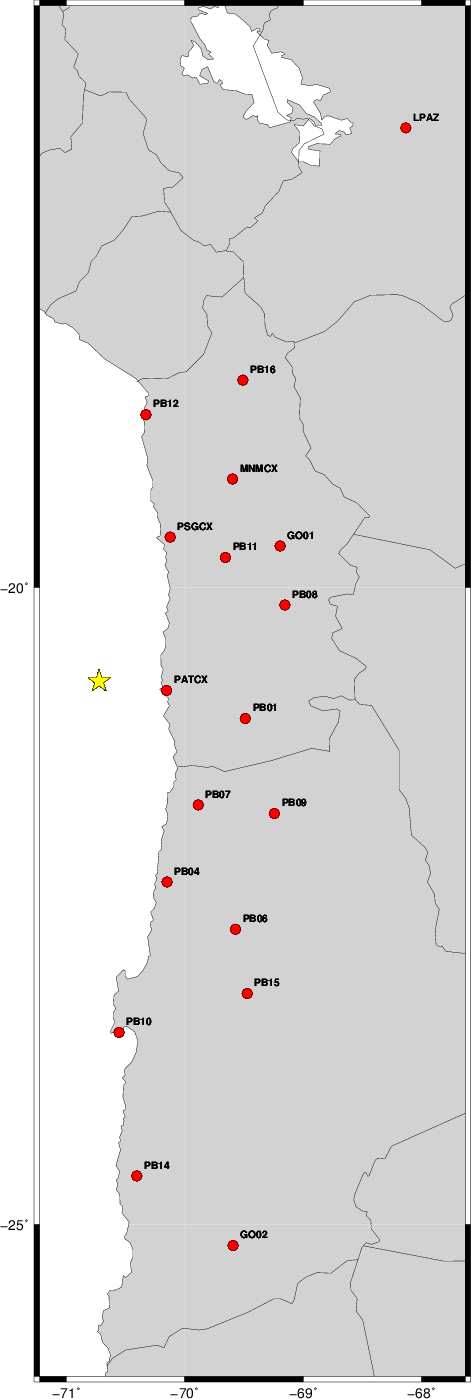
Waveform Inversion
The focal mechanism was determined using broadband seismic waveforms. The location of the event and the
and stations used for the waveform inversion are shown in the next figure.
|
|
Location of broadband stations used for waveform inversion
|
The program wvfgrd96 was used with good traces observed at short distance to determine the focal mechanism, depth and seismic moment. This technique requires a high quality signal and well determined velocity model for the Green functions. To the extent that these are the quality data, this type of mechanism should be preferred over the radiation pattern technique which requires the separate step of defining the pressure and tension quadrants and the correct strike.
The observed and predicted traces are filtered using the following gsac commands:
cut a -30 a 180
rtr
taper w 0.1
hp c 0.02 n 3
lp c 0.06 n 3
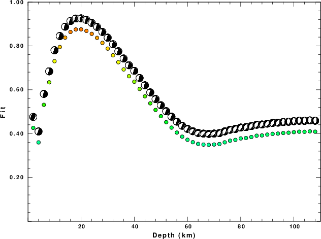
The results of this grid search from 0.5 to 19 km depth are as follow:
           DEPTH  STK   DIP  RAKE   MW    FIT
WVFGRD96    2.0   200    40    90   5.74 0.4259
WVFGRD96    4.0   305    15    15   5.82 0.3597
WVFGRD96    6.0   300    15    15   5.84 0.5311
WVFGRD96    8.0   305    10    20   5.92 0.6339
WVFGRD96   10.0   315    15    30   5.92 0.7300
WVFGRD96   12.0   320    20    35   5.94 0.7949
WVFGRD96   14.0   325    20    40   5.95 0.8376
WVFGRD96   16.0   325    25    40   5.96 0.8634
WVFGRD96   18.0   320    25    35   5.97 0.8749
WVFGRD96   20.0   320    25    35   5.98 0.8755
WVFGRD96   22.0   320    25    35   6.00 0.8684
WVFGRD96   24.0   315    25    30   6.02 0.8549
WVFGRD96   26.0   315    25    30   6.03 0.8366
WVFGRD96   28.0   310    25    25   6.04 0.8138
WVFGRD96   30.0   310    25    25   6.05 0.7875
WVFGRD96   32.0   310    25    25   6.06 0.7574
WVFGRD96   34.0   310    25    25   6.07 0.7255
WVFGRD96   36.0   305    25    20   6.07 0.6926
WVFGRD96   38.0   305    25    20   6.07 0.6618
WVFGRD96   40.0   305    20    20   6.21 0.6364
WVFGRD96   42.0   305    20    20   6.22 0.6036
WVFGRD96   44.0   305    20    20   6.22 0.5703
WVFGRD96   46.0   300    20    15   6.23 0.5380
WVFGRD96   48.0   295    25     5   6.23 0.5078
WVFGRD96   50.0   295    25     5   6.24 0.4793
WVFGRD96   52.0   290    25     0   6.24 0.4521
WVFGRD96   54.0   290    25     0   6.24 0.4273
WVFGRD96   56.0   285    25    -5   6.24 0.4046
WVFGRD96   58.0   280    25   -15   6.24 0.3858
WVFGRD96   60.0   275    25   -25   6.25 0.3717
WVFGRD96   62.0   275    30   -30   6.25 0.3608
WVFGRD96   64.0   265    30   -45   6.25 0.3529
WVFGRD96   66.0   260    30   -50   6.26 0.3498
WVFGRD96   68.0   265    35   -50   6.26 0.3486
WVFGRD96   70.0   260    35   -55   6.27 0.3501
WVFGRD96   72.0   220    35   -75   6.27 0.3523
WVFGRD96   74.0   220    35   -75   6.28 0.3601
WVFGRD96   76.0   220    35   -75   6.29 0.3675
WVFGRD96   78.0   220    35   -75   6.29 0.3713
WVFGRD96   80.0   220    35   -75   6.30 0.3777
WVFGRD96   82.0   215    35   -80   6.31 0.3797
WVFGRD96   84.0   215    35   -80   6.31 0.3842
WVFGRD96   86.0   215    35   -80   6.32 0.3903
WVFGRD96   88.0   215    35   -80   6.32 0.3915
WVFGRD96   90.0   220    40   -80   6.32 0.3953
WVFGRD96   92.0   215    40   -80   6.33 0.3986
WVFGRD96   94.0   215    40   -80   6.33 0.4000
WVFGRD96   96.0    10    50   -80   6.33 0.4026
WVFGRD96   98.0    10    50   -80   6.33 0.4039
WVFGRD96  100.0    10    50   -80   6.34 0.4065
WVFGRD96  102.0    10    50   -80   6.34 0.4085
WVFGRD96  104.0    10    50   -80   6.34 0.4081
WVFGRD96  106.0    10    50   -80   6.35 0.4100
WVFGRD96  108.0    10    50   -80   6.35 0.4086
The best solution is
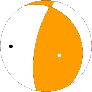
WVFGRD96 20.0 320 25 35 5.98 0.8755
The mechanism correspond to the best fit is
|
|
Figure 1. Waveform inversion focal mechanism
|
The best fit as a function of depth is given in the following figure:
|
|
Figure 2. Depth sensitivity for waveform mechanism
|
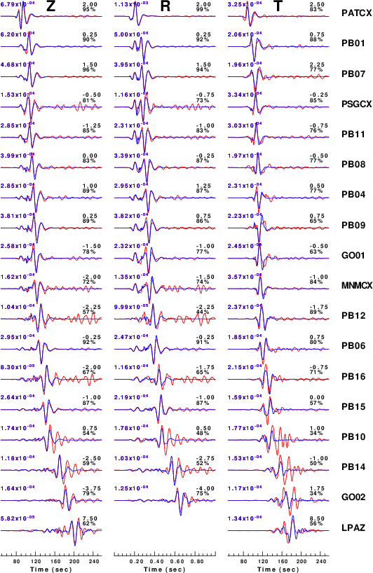
The comparison of the observed and predicted waveforms is given in the next figure. The red traces are the observed and the blue are the predicted.
Each observed-predicted component is plotted to the same scale and peak amplitudes are indicated by the numbers to the left of each trace. A pair of numbers is given in black at the right of each predicted traces. The upper number it the time shift required for maximum correlation between the observed and predicted traces. This time shift is required because the synthetics are not computed at exactly the same distance as the observed and because the velocity model used in the predictions may not be perfect.
A positive time shift indicates that the prediction is too fast and should be delayed to match the observed trace (shift to the right in this figure). A negative value indicates that the prediction is too slow. The lower number gives the percentage of variance reduction to characterize the individual goodness of fit (100% indicates a perfect fit).
The bandpass filter used in the processing and for the display was
cut a -30 a 180
rtr
taper w 0.1
hp c 0.02 n 3
lp c 0.06 n 3
|
|
Figure 3. Waveform comparison for selected depth. Red: observed; Blue - predicted. The time shift with respect to the model prediction is indicated. The percent of fit is also indicated.
|
|
|
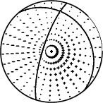
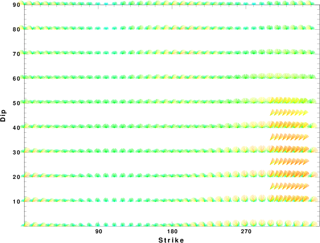
Focal mechanism sensitivity at the preferred depth. The red color indicates a very good fit to thewavefroms.
Each solution is plotted as a vector at a given value of strike and dip with the angle of the vector representing the rake angle, measured, with respect to the upward vertical (N) in the figure.
|
A check on the assumed source location is possible by looking at the time shifts between the observed and predicted traces. The time shifts for waveform matching arise for several reasons:
- The origin time and epicentral distance are incorrect
- The velocity model used for the inversion is incorrect
- The velocity model used to define the P-arrival time is not the
same as the velocity model used for the waveform inversion
(assuming that the initial trace alignment is based on the
P arrival time)
Assuming only a mislocation, the time shifts are fit to a functional form:
Time_shift = A + B cos Azimuth + C Sin Azimuth
The time shifts for this inversion lead to the next figure:
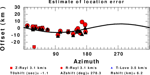
The derived shift in origin time and epicentral coordinates are given at the bottom of the figure.
Discussion
Acknowledgements
Thanks also to the many seismic network operators whose dedication make this effort possible: University of Nevada Reno, University of Alaska, University of Washington, Oregon State University, University of Utah, Montana Bureas of Mines, UC Berkely, Caltech, UC San Diego, Saint Louis University, University of Memphis, Lamont Doherty Earth Observatory, the Iris stations and the Transportable Array of EarthScope.
Velocity Model
The WUS used for the waveform synthetic seismograms and for the surface wave eigenfunctions and dispersion is as follows:
MODEL.01
Model after     8 iterations
ISOTROPIC
KGS
FLAT EARTH
1-D
CONSTANT VELOCITY
LINE08
LINE09
LINE10
LINE11
      H(KM)   VP(KM/S)   VS(KM/S) RHO(GM/CC)         QP         QS       ETAP       ETAS      FREFP      FREFS
     1.9000     3.4065     2.0089     2.2150  0.302E-02  0.679E-02   0.00       0.00       1.00       1.00
     6.1000     5.5445     3.2953     2.6089  0.349E-02  0.784E-02   0.00       0.00       1.00       1.00
    13.0000     6.2708     3.7396     2.7812  0.212E-02  0.476E-02   0.00       0.00       1.00       1.00
    19.0000     6.4075     3.7680     2.8223  0.111E-02  0.249E-02   0.00       0.00       1.00       1.00
     0.0000     7.9000     4.6200     3.2760  0.164E-10  0.370E-10   0.00       0.00       1.00       1.00
Quality Control
Here we tabulate the reasons for not using certain digital data sets
The following stations did not have a valid response files:
Last Changed Fri Apr 11 11:53:04 CDT 2014