2012/05/12 23:28:43 38.658 70.414 10.0 5.70 Tadjikistan
USGS Felt map for this earthquake
 USGS/SLU Moment Tensor Solution
 ENS  2012/05/12 23:28:43:7  38.66   70.41  10.0 5.7 Tadjikistan

 Stations used:
   II.AAK II.NIL IU.KBL KR.KDJ KR.NRN

 Filtering commands used:
   hp c 0.015 n 3
   lp c 0.033 n 3

 Best Fitting Double Couple
  Mo = 3.16e+24 dyne-cm
  Mw = 5.60
  Z  = 25 km
  Plane   Strike  Dip  Rake
   NP1      190    75    60
   NP2       76    33   152
  Principal Axes:
   Axis    Value   Plunge  Azimuth
    T   3.16e+24     51      66
    N   0.00e+00     29     198
    P  -3.16e+24     24     303

 Moment Tensor: (dyne-cm)
    Component   Value
       Mxx    -5.64e+23
       Mxy     1.67e+24
       Mxz    -8.83e+21
       Myy    -8.06e+23
       Myz     2.41e+24
       Mzz     1.37e+24


                     ----------####
                 -------------#########
              ---------------#############
             ---------------###############
           ----------------##################
          ---   -----------###################
         ---- P ----------#####################
        -----   ---------###########   #########
        -----------------########### T #########
       ------------------###########   #########-
       -----------------#######################--
       -----------------#######################--
       -----------------######################---
        ---------------######################---
        #--------------####################-----
         #-------------##################------
          ###----------################-------
           #####-------#############---------
             ########--#######-------------
              #########-------------------
                 #######---------------
                     ###-----------


 Global CMT Convention Moment Tensor:
      R          T          P
  1.37e+24  -8.83e+21  -2.41e+24
 -8.83e+21  -5.64e+23  -1.67e+24
 -2.41e+24  -1.67e+24  -8.06e+23


Details of the solution is found at

http://www.eas.slu.edu/Earthquake_Center/MECH.NA/20120512232843/index.html
|
      STK = 190
      DIP = 75
     RAKE = 60
       MW = 5.60
       HS = 25.0
The waveform inversion is preferred.
The following compares this source inversion to others
 USGS/SLU Moment Tensor Solution
 ENS  2012/05/12 23:28:43:7  38.66   70.41  10.0 5.7 Tadjikistan

 Stations used:
   II.AAK II.NIL IU.KBL KR.KDJ KR.NRN

 Filtering commands used:
   hp c 0.015 n 3
   lp c 0.033 n 3

 Best Fitting Double Couple
  Mo = 3.16e+24 dyne-cm
  Mw = 5.60
  Z  = 25 km
  Plane   Strike  Dip  Rake
   NP1      190    75    60
   NP2       76    33   152
  Principal Axes:
   Axis    Value   Plunge  Azimuth
    T   3.16e+24     51      66
    N   0.00e+00     29     198
    P  -3.16e+24     24     303

 Moment Tensor: (dyne-cm)
    Component   Value
       Mxx    -5.64e+23
       Mxy     1.67e+24
       Mxz    -8.83e+21
       Myy    -8.06e+23
       Myz     2.41e+24
       Mzz     1.37e+24


                     ----------####
                 -------------#########
              ---------------#############
             ---------------###############
           ----------------##################
          ---   -----------###################
         ---- P ----------#####################
        -----   ---------###########   #########
        -----------------########### T #########
       ------------------###########   #########-
       -----------------#######################--
       -----------------#######################--
       -----------------######################---
        ---------------######################---
        #--------------####################-----
         #-------------##################------
          ###----------################-------
           #####-------#############---------
             ########--#######-------------
              #########-------------------
                 #######---------------
                     ###-----------


 Global CMT Convention Moment Tensor:
      R          T          P
  1.37e+24  -8.83e+21  -2.41e+24
 -8.83e+21  -5.64e+23  -1.67e+24
 -2.41e+24  -1.67e+24  -8.06e+23


Details of the solution is found at

http://www.eas.slu.edu/Earthquake_Center/MECH.NA/20120512232843/index.html
|
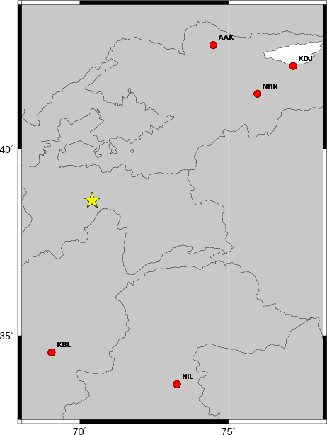
The focal mechanism was determined using broadband seismic waveforms. The location of the event and the and stations used for the waveform inversion are shown in the next figure.
|
|
|
|
The program wvfgrd96 was used with good traces observed at short distance to determine the focal mechanism, depth and seismic moment. This technique requires a high quality signal and well determined velocity model for the Green functions. To the extent that these are the quality data, this type of mechanism should be preferred over the radiation pattern technique which requires the separate step of defining the pressure and tension quadrants and the correct strike.
The observed and predicted traces are filtered using the following gsac commands:
hp c 0.015 n 3
lp c 0.033 n 3
The results of this grid search from 0.5 to 19 km depth are as follow:
           DEPTH  STK   DIP  RAKE   MW    FIT
WVFGRD96    1.0   265    75   -15   5.31 0.4343
WVFGRD96    2.0   265    70   -10   5.35 0.4434
WVFGRD96    3.0   265    50     0   5.41 0.4387
WVFGRD96    4.0   265    40     0   5.46 0.4367
WVFGRD96    5.0   265    35     0   5.49 0.4403
WVFGRD96    6.0   265    30     0   5.51 0.4477
WVFGRD96    7.0   265    25    -5   5.53 0.4569
WVFGRD96    8.0   260    20   -15   5.60 0.4668
WVFGRD96    9.0   250    15   -30   5.62 0.4858
WVFGRD96   10.0   240    15   -45   5.63 0.5048
WVFGRD96   11.0   195    80    80   5.62 0.5262
WVFGRD96   12.0   195    80    80   5.62 0.5445
WVFGRD96   13.0   195    80    80   5.61 0.5574
WVFGRD96   14.0   190    80    75   5.60 0.5726
WVFGRD96   15.0   190    80    75   5.60 0.5832
WVFGRD96   16.0   190    80    70   5.59 0.5935
WVFGRD96   17.0   190    80    70   5.59 0.6024
WVFGRD96   18.0   190    80    70   5.59 0.6095
WVFGRD96   19.0   195    75    70   5.60 0.6165
WVFGRD96   20.0   190    80    65   5.59 0.6212
WVFGRD96   21.0   190    75    65   5.60 0.6274
WVFGRD96   22.0   190    75    65   5.60 0.6309
WVFGRD96   23.0   190    75    60   5.60 0.6337
WVFGRD96   24.0   190    75    60   5.60 0.6371
WVFGRD96   25.0   190    75    60   5.60 0.6378
WVFGRD96   26.0   190    75    60   5.61 0.6372
WVFGRD96   27.0   190    75    60   5.61 0.6377
WVFGRD96   28.0   190    75    55   5.61 0.6357
WVFGRD96   29.0   190    75    55   5.61 0.6333
WVFGRD96   30.0   190    75    55   5.61 0.6316
WVFGRD96   31.0   185    75    50   5.61 0.6283
WVFGRD96   32.0   185    75    50   5.61 0.6256
WVFGRD96   33.0   185    75    50   5.62 0.6205
WVFGRD96   34.0   185    75    50   5.62 0.6154
WVFGRD96   35.0   185    75    50   5.62 0.6106
WVFGRD96   36.0   190    75    55   5.62 0.6045
WVFGRD96   37.0   190    75    55   5.62 0.5982
WVFGRD96   38.0   190    75    55   5.62 0.5920
WVFGRD96   39.0   190    75    55   5.62 0.5851
WVFGRD96   40.0   190    70    60   5.75 0.6044
WVFGRD96   41.0   190    70    60   5.76 0.5973
WVFGRD96   42.0   190    70    60   5.76 0.5898
WVFGRD96   43.0   190    70    60   5.76 0.5820
WVFGRD96   44.0   190    70    55   5.76 0.5743
WVFGRD96   45.0   190    70    55   5.77 0.5665
WVFGRD96   46.0   190    70    55   5.77 0.5586
WVFGRD96   47.0   190    70    55   5.77 0.5505
WVFGRD96   48.0   185    75    45   5.77 0.5424
WVFGRD96   49.0   185    75    45   5.77 0.5349
WVFGRD96   50.0   185    75    45   5.78 0.5273
WVFGRD96   51.0   185    75    45   5.78 0.5195
WVFGRD96   52.0   185    75    45   5.78 0.5117
WVFGRD96   53.0   185    75    45   5.79 0.5038
WVFGRD96   54.0   185    75    45   5.79 0.4959
WVFGRD96   55.0   185    75    45   5.79 0.4869
WVFGRD96   56.0   185    75    45   5.79 0.4790
WVFGRD96   57.0   185    75    40   5.80 0.4712
WVFGRD96   58.0   185    75    40   5.80 0.4636
WVFGRD96   59.0   185    75    40   5.80 0.4559
WVFGRD96   60.0   185    75    40   5.81 0.4482
WVFGRD96   61.0   185    75    40   5.81 0.4406
WVFGRD96   62.0   185    75    40   5.81 0.4330
WVFGRD96   63.0   185    75    40   5.81 0.4254
WVFGRD96   64.0   185    75    40   5.82 0.4179
WVFGRD96   65.0   185    75    40   5.82 0.4104
WVFGRD96   66.0   185    75    40   5.82 0.4019
WVFGRD96   67.0   185    75    40   5.82 0.3946
WVFGRD96   68.0   185    75    40   5.83 0.3873
WVFGRD96   69.0   185    75    40   5.83 0.3802
WVFGRD96   70.0   185    75    40   5.83 0.3730
WVFGRD96   71.0   185    75    40   5.83 0.3660
WVFGRD96   72.0   185    75    40   5.83 0.3590
WVFGRD96   73.0   185    75    40   5.84 0.3521
WVFGRD96   74.0   185    75    40   5.84 0.3453
WVFGRD96   75.0   185    75    40   5.84 0.3386
WVFGRD96   76.0   185    75    40   5.84 0.3320
WVFGRD96   77.0   185    75    40   5.84 0.3254
WVFGRD96   78.0   185    75    40   5.85 0.3189
WVFGRD96   79.0   185    75    40   5.85 0.3125
WVFGRD96   80.0   185    75    40   5.85 0.3061
WVFGRD96   81.0   185    75    45   5.85 0.2998
WVFGRD96   82.0   185    75    45   5.85 0.2937
WVFGRD96   83.0   185    75    45   5.85 0.2876
WVFGRD96   84.0   185    75    45   5.85 0.2816
WVFGRD96   85.0   185    75    45   5.86 0.2757
WVFGRD96   86.0   185    75    45   5.86 0.2699
WVFGRD96   87.0   185    75    45   5.86 0.2641
WVFGRD96   88.0   185    75    45   5.86 0.2585
WVFGRD96   89.0   185    75    45   5.86 0.2521
WVFGRD96   90.0   185    75    45   5.86 0.2466
WVFGRD96   91.0   185    75    45   5.86 0.2406
WVFGRD96   92.0   185    75    45   5.86 0.2352
WVFGRD96   93.0   185    75    45   5.87 0.2299
WVFGRD96   94.0   185    75    50   5.86 0.2247
WVFGRD96   95.0   185    75    50   5.87 0.2197
WVFGRD96   96.0   185    75    50   5.87 0.2147
WVFGRD96   97.0   185    75    50   5.87 0.2097
WVFGRD96   98.0   185    75    50   5.87 0.2048
WVFGRD96   99.0   185    75    50   5.87 0.2000
The best solution is
WVFGRD96 25.0 190 75 60 5.60 0.6378
The mechanism correspond to the best fit is
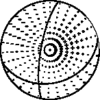
|
|
|
The best fit as a function of depth is given in the following figure:
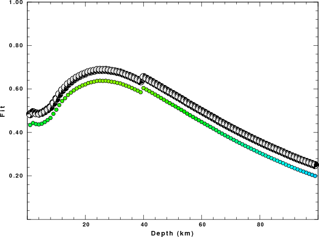
|
|
|
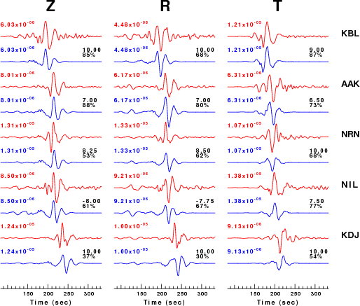
The comparison of the observed and predicted waveforms is given in the next figure. The red traces are the observed and the blue are the predicted. Each observed-predicted component is plotted to the same scale and peak amplitudes are indicated by the numbers to the left of each trace. A pair of numbers is given in black at the right of each predicted traces. The upper number it the time shift required for maximum correlation between the observed and predicted traces. This time shift is required because the synthetics are not computed at exactly the same distance as the observed and because the velocity model used in the predictions may not be perfect. A positive time shift indicates that the prediction is too fast and should be delayed to match the observed trace (shift to the right in this figure). A negative value indicates that the prediction is too slow. The lower number gives the percentage of variance reduction to characterize the individual goodness of fit (100% indicates a perfect fit).
The bandpass filter used in the processing and for the display was
hp c 0.015 n 3
lp c 0.033 n 3
|
|
|
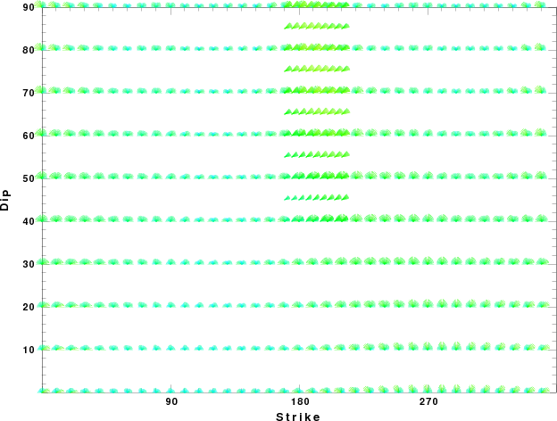
|
| Focal mechanism sensitivity at the preferred depth. The red color indicates a very good fit to thewavefroms. Each solution is plotted as a vector at a given value of strike and dip with the angle of the vector representing the rake angle, measured, with respect to the upward vertical (N) in the figure. |
A check on the assumed source location is possible by looking at the time shifts between the observed and predicted traces. The time shifts for waveform matching arise for several reasons:
Time_shift = A + B cos Azimuth + C Sin Azimuth
The time shifts for this inversion lead to the next figure:
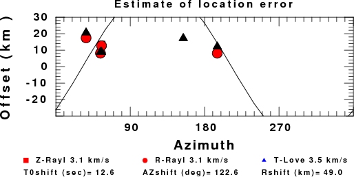
The derived shift in origin time and epicentral coordinates are given at the bottom of the figure.
Should the national backbone of the USGS Advanced National Seismic System (ANSS) be implemented with an interstation separation of 300 km, it is very likely that an earthquake such as this would have been recorded at distances on the order of 100-200 km. This means that the closest station would have information on source depth and mechanism that was lacking here.
Dr. Harley Benz, USGS, provided the USGS USNSN digital data. The digital data used in this study were provided by Natural Resources Canada through their AUTODRM site http://www.seismo.nrcan.gc.ca/nwfa/autodrm/autodrm_req_e.php, and IRIS using their BUD interface.
Thanks also to the many seismic network operators whose dedication make this effort possible: University of Alaska, University of Washington, Oregon State University, University of Utah, Montana Bureas of Mines, UC Berkely, Caltech, UC San Diego, Saint L ouis University, Universityof Memphis, Lamont Doehrty Earth Observatory, Boston College, the Iris stations and the Transportable Array of EarthScope.
The WUS used for the waveform synthetic seismograms and for the surface wave eigenfunctions and dispersion is as follows:
MODEL.01
Model after     8 iterations
ISOTROPIC
KGS
FLAT EARTH
1-D
CONSTANT VELOCITY
LINE08
LINE09
LINE10
LINE11
      H(KM)   VP(KM/S)   VS(KM/S) RHO(GM/CC)         QP         QS       ETAP       ETAS      FREFP      FREFS
     1.9000     3.4065     2.0089     2.2150  0.302E-02  0.679E-02   0.00       0.00       1.00       1.00
     6.1000     5.5445     3.2953     2.6089  0.349E-02  0.784E-02   0.00       0.00       1.00       1.00
    13.0000     6.2708     3.7396     2.7812  0.212E-02  0.476E-02   0.00       0.00       1.00       1.00
    19.0000     6.4075     3.7680     2.8223  0.111E-02  0.249E-02   0.00       0.00       1.00       1.00
     0.0000     7.9000     4.6200     3.2760  0.164E-10  0.370E-10   0.00       0.00       1.00       1.00
Here we tabulate the reasons for not using certain digital data sets
The following stations did not have a valid response files:
DATE=Sat May 12 18:29:30 MDT 2012