Location
SMU Location
2007/08/24 07:45:22 40.5500 123.033 10.0 3.70
SLU Location - Preferred
The SMU location could not fit the P-wave first motion on the Z and R components at station YLING. Interestingly the strongest arrival is the Transverse componet. In addition the waveform inversion required a set of positive time shifts. The preferred solution is from elocate and is given in detail in elocate.txt has an origin time about 2 seconds later than the SMU solution. Perhaps this is because of the use of the sharp S-wave arrivals.
As you can see from the plots YLING is not fit well - the solution at a close station depends upon azimuth very strongly. Fortunately the distance weighting used downweights YLING so that it does not affect the solution. The solution without YLING is
WVFGRD96 8.0 275 70 -25 3.81 0.7907
The SLU location is as follows:
2007/08/24 07:45:24 40.5300 123.064 18.0 3.70
Arrival Times (from USGS)
Arrival time list
Felt Map
USGS Felt map for this earthquake
USGS Felt reports page for
Focal Mechanism
 USGS/SLU Moment Tensor Solution
 ENS  2007/08/24 07:45:24:2  40.53  123.06  18.0 3.7

 Stations used:
   XG.HGOU XG.HQI XG.LJIA XG.MJD XG.WTANG XG.XDIAN XG.YLING

 Filtering commands used:
   hp c 0.05 n 3
   lp c 0.50 n 3

 Best Fitting Double Couple
  Mo = 5.89e+21 dyne-cm
  Mw = 3.78
  Z  = 8 km
  Plane   Strike  Dip  Rake
   NP1      275    70   -25
   NP2       14    67   -158
  Principal Axes:
   Axis    Value   Plunge  Azimuth
    T   5.89e+21      2     325
    N   0.00e+00     58      59
    P  -5.89e+21     32     234

 Moment Tensor: (dyne-cm)
    Component   Value
       Mxx     2.46e+21
       Mxy    -4.80e+21
       Mxz     1.74e+21
       Myy    -8.59e+20
       Myz     1.98e+21
       Mzz    -1.60e+21


                     ############--
                 T ###############-----
              ##   ################-------
             ######################--------
           ########################----------
          #########################-----------
         ##########################------------
        ###########################-------------
        #######-----------------###-------------
       ##--------------------------#####---------
       ---------------------------###########----
       ---------------------------##############-
       --------------------------################
        -------------------------###############
        -------   --------------################
         ------ P -------------################
          -----   -------------###############
           -------------------###############
             ----------------##############
              -------------###############
                 ---------#############
                     ---###########


 Global CMT Convention Moment Tensor:
      R          T          P
 -1.60e+21   1.74e+21  -1.98e+21
  1.74e+21   2.46e+21   4.80e+21
 -1.98e+21   4.80e+21  -8.59e+20


Details of the solution is found at

http://www.eas.slu.edu/Earthquake_Center/MECH.NA/20070824074524/index.html
|
Preferred Solution
The preferred solution from an analysis of the surface-wave spectral amplitude radiation pattern, waveform inversion and first motion observations is
      STK = 275
      DIP = 70
     RAKE = -25
       MW = 3.78
       HS = 8.0
The waveform inversion is preferred.
Moment Tensor Comparison
The following compares this source inversion to others
| SLU |
SLU |
 USGS/SLU Moment Tensor Solution
 ENS  2007/08/24 07:45:24:2  40.53  123.06  18.0 3.7

 Stations used:
   XG.HGOU XG.HQI XG.LJIA XG.MJD XG.WTANG XG.XDIAN XG.YLING

 Filtering commands used:
   hp c 0.05 n 3
   lp c 0.50 n 3

 Best Fitting Double Couple
  Mo = 5.89e+21 dyne-cm
  Mw = 3.78
  Z  = 8 km
  Plane   Strike  Dip  Rake
   NP1      275    70   -25
   NP2       14    67   -158
  Principal Axes:
   Axis    Value   Plunge  Azimuth
    T   5.89e+21      2     325
    N   0.00e+00     58      59
    P  -5.89e+21     32     234

 Moment Tensor: (dyne-cm)
    Component   Value
       Mxx     2.46e+21
       Mxy    -4.80e+21
       Mxz     1.74e+21
       Myy    -8.59e+20
       Myz     1.98e+21
       Mzz    -1.60e+21


                     ############--
                 T ###############-----
              ##   ################-------
             ######################--------
           ########################----------
          #########################-----------
         ##########################------------
        ###########################-------------
        #######-----------------###-------------
       ##--------------------------#####---------
       ---------------------------###########----
       ---------------------------##############-
       --------------------------################
        -------------------------###############
        -------   --------------################
         ------ P -------------################
          -----   -------------###############
           -------------------###############
             ----------------##############
              -------------###############
                 ---------#############
                     ---###########


 Global CMT Convention Moment Tensor:
      R          T          P
 -1.60e+21   1.74e+21  -1.98e+21
  1.74e+21   2.46e+21   4.80e+21
 -1.98e+21   4.80e+21  -8.59e+20


Details of the solution is found at

http://www.eas.slu.edu/Earthquake_Center/MECH.NA/20070824074524/index.html
|
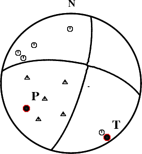
This is a plot of observed first motions together with the
waveform grid search nodal planes:
|
Waveform Inversion
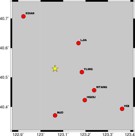
The focal mechanism was determined using broadband seismic waveforms. The location of the event and the
and stations used for the waveform inversion are shown in the next figure.
|
|
Location of broadband stations used for waveform inversion
|
The program wvfgrd96 was used with good traces observed at short distance to determine the focal mechanism, depth and seismic moment. This technique requires a high quality signal and well determined velocity model for the Green functions. To the extent that these are the quality data, this type of mechanism should be preferred over the radiation pattern technique which requires the separate step of defining the pressure and tension quadrants and the correct strike.
The observed and predicted traces are filtered using the following gsac commands:
hp c 0.05 n 3
lp c 0.50 n 3
The results of this grid search from 0.5 to 19 km depth are as follow:
           DEPTH  STK   DIP  RAKE   MW    FIT
WVFGRD96    0.5    10    90   -20   3.46 0.4556
WVFGRD96    1.0   275    65   -30   3.55 0.4849
WVFGRD96    2.0   105    75    20   3.58 0.5152
WVFGRD96    3.0   280    75   -15   3.63 0.5286
WVFGRD96    4.0   280    75   -15   3.67 0.5405
WVFGRD96    5.0   280    70   -15   3.70 0.5662
WVFGRD96    6.0   280    70   -20   3.73 0.5904
WVFGRD96    7.0   275    65   -25   3.76 0.6185
WVFGRD96    8.0   275    70   -25   3.78 0.6272
WVFGRD96    9.0   275    70   -25   3.80 0.6166
WVFGRD96   10.0   275    70   -30   3.81 0.5943
WVFGRD96   11.0   275    70   -30   3.83 0.5794
WVFGRD96   12.0   280    80   -20   3.84 0.5562
WVFGRD96   13.0   280    80   -20   3.85 0.5399
WVFGRD96   14.0   280    80   -15   3.86 0.5309
WVFGRD96   15.0   280    80   -15   3.87 0.4979
WVFGRD96   16.0   105    90    10   3.89 0.5119
WVFGRD96   17.0   105    90    10   3.90 0.5140
WVFGRD96   18.0   285    90   -10   3.91 0.5023
WVFGRD96   19.0   285    90   -10   3.93 0.5203
WVFGRD96   20.0   105    90    15   3.94 0.5239
WVFGRD96   21.0   105    90    10   3.97 0.5239
WVFGRD96   22.0   105    90    15   3.96 0.5052
WVFGRD96   23.0   285    90   -10   3.99 0.5117
WVFGRD96   24.0   105    85    15   4.00 0.5182
WVFGRD96   25.0   105    90    10   4.02 0.5196
WVFGRD96   26.0   105    90    10   4.03 0.5135
WVFGRD96   27.0   105    75    25   4.02 0.4937
WVFGRD96   28.0   105    75    25   4.03 0.4962
WVFGRD96   29.0   105    75    20   4.05 0.4957
The best solution is
WVFGRD96 8.0 275 70 -25 3.78 0.6272
The mechanism correspond to the best fit is
|
|
Figure 1. Waveform inversion focal mechanism
|
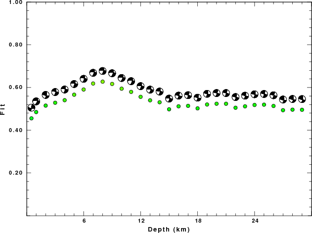
The best fit as a function of depth is given in the following figure:
|
|
Figure 2. Depth sensitivity for waveform mechanism
|
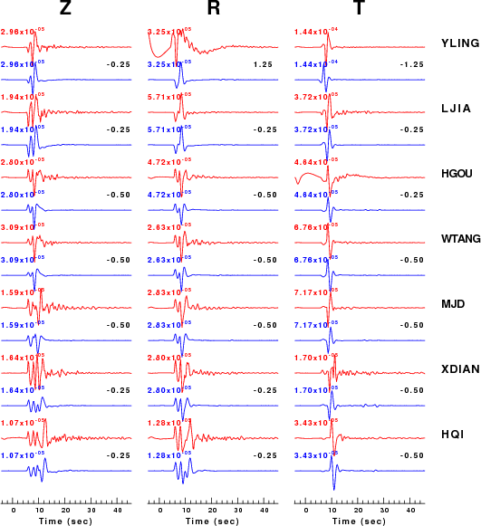
The comparison of the observed and predicted waveforms is given in the next figure. The red traces are the observed and the blue are the predicted.
Each observed-predicted componnet is plotted to the same scale and peak amplitudes are indicated by the numbers to the left of each trace. The number in black at the rightr of each predicted traces it the time shift required for maximum correlation between the observed and predicted traces. This time shift is required because the synthetics are not computed at exactly the same distance as the observed and because the velocity model used in the predictions may not be perfect.
A positive time shift indicates that the prediction is too fast and should be delayed to match the observed trace (shift to the right in this figure). A negative value indicates that the prediction is too slow.
The bandpass filter used in the processing and for the display was
hp c 0.05 n 3
lp c 0.50 n 3
|
|
Figure 3. Waveform comparison for selected depth
|
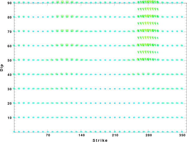
|
|
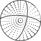
Focal mechanism sensitivity at the preferred depth. The red color indicates a very good fit to thewavefroms.
Each solution is plotted as a vector at a given value of strike and dip with the angle of the vector representing the rake angle, measured, with respect to the upward vertical (N) in the figure.
|
Discussion
The Future
Should the national backbone of the
USGS Advanced National Seismic System (ANSS)
be implemented with an interstation separation of 300 km, it is very likely that
an earthquake such as this would have been recorded at distances on the order of
100-200 km. This means that the closest station would have information on
source depth and mechanism that was lacking here.
Acknowledgements
Dr. Harley Benz, USGS, provided the USGS USNSN digital data.
The digital data used in this study were provided by Natural Resources Canada through their AUTODRM site http://www.seismo.nrcan.gc.ca/nwfa/autodrm/autodrm_req_e.php, and IRIS using their BUD interface.
Thanks also to the many seismic network operators whose dedication make this effort possible: University of Alaska, University of Washington, Oregon State University, University of Utah, Montana Bureas of Mines, UC Berkely, Caltech, UC San Diego, Saint L ouis University, Universityof Memphis, Lamont Doehrty Earth Observatory, Boston College, the Iris stations and the Transportable Array of EarthScope.
Velocity Model
The CUS used for the waveform synthetic seismograms and for the surface wave eigenfunctions and dispersion is as follows:
MODEL.01
CUS Model with Q from simple gamma values
ISOTROPIC
KGS
FLAT EARTH
1-D
CONSTANT VELOCITY
LINE08
LINE09
LINE10
LINE11
  H(KM) VP(KM/S) VS(KM/S) RHO(GM/CC)   QP   QS  ETAP  ETAS  FREFP  FREFS
  1.0000  5.0000  2.8900  2.5000 0.172E-02 0.387E-02 0.00  0.00  1.00  1.00
  9.0000  6.1000  3.5200  2.7300 0.160E-02 0.363E-02 0.00  0.00  1.00  1.00
 10.0000  6.4000  3.7000  2.8200 0.149E-02 0.336E-02 0.00  0.00  1.00  1.00
 20.0000  6.7000  3.8700  2.9020 0.000E-04 0.000E-04 0.00  0.00  1.00  1.00
  0.0000  8.1500  4.7000  3.3640 0.194E-02 0.431E-02 0.00  0.00  1.00  1.00
Quality Control
Here we tabulate the reasons for not using certain digital data sets
The following stations did not have a valid response files:
DATE=Thu May 20 22:53:47 CDT 2010
Last Changed 2007/08/24