Location

2013/06/09 14:22:12 -25.967 131.976 1.1 5.8 Australia

The Earthquakes@Geoscience Australia solution is http://www.ga.gov.au/earthquakes/getQuakeTechController.do?orid=772311&quakeId=3373820

Magnitude	Location (uncertainty)
Mwp: Not available	Latitude: -25.857 (+/- 0.6482km)
Mb: Not available	Longitude: 131.842 (+/- 0.5274km)
Ms: (Not available)	Depth: 0 km (+/- 3.6168km)
Md: Not available	 
ML: 5.7	 (Preferred)	 
 	 
Quality indicators	Solution status
Number of stations used: 27 (of 55 possible)	Last updated: 10 June 2013 @ 12:41:12 (AEST)
Number of phase used: 27 (of 67 possible)	Finalised: No
Gap angles: 60°	Source: AUST
RMS residual: 5.19 seconds	

Arrival Times (from USGS)

Arrival time list

Felt Map

USGS Felt map for this earthquake USGS Felt map for this earthquake

USGS Felt reports main page

Focal Mechanism

USGS/SLU Moment Tensor Solution ENS 2013/06/09 14:22:12:0 -25.97 131.98 1.1 5.8 Australia Stations used: AU.BBOO AU.FORT AU.HTT AU.KMBL AU.KNRA AU.QIS AU.STKA AU.WB2 AU.WC3 AU.WRKA II.WRAB Filtering commands used: hp c 0.01 n 3 lp c 0.05 n 3 Best Fitting Double Couple Mo = 1.76e+24 dyne-cm Mw = 5.43 Z = 2 km Plane Strike Dip Rake NP1 280 60 55 NP2 154 45 135 Principal Axes: Axis Value Plunge Azimuth T 1.76e+24 59 138 N 0.00e+00 30 299 P -1.76e+24 9 34 Moment Tensor: (dyne-cm) Component Value Mxx -9.11e+23 Mxy -1.03e+24 Mxz -7.97e+23 Myy -3.36e+23 Myz 3.71e+23 Mzz 1.25e+24 -------------- #------------------- ###-------------------- P -- ###--------------------- --- #####----------------------------- #####------------------------------- ######-------------------------------- #####--###################-------------- #------########################--------- --------###########################------- ---------############################----- ---------##############################--- ----------###############################- ----------############## ############# -----------############# T ############# -----------############ ############ -----------######################### ------------###################### ------------################## -------------############### --------------######## -------------- Global CMT Convention Moment Tensor: R T P 1.25e+24 -7.97e+23 -3.71e+23 -7.97e+23 -9.11e+23 1.03e+24 -3.71e+23 1.03e+24 -3.36e+23 Details of the solution is found at http://www.eas.slu.edu/Earthquake_Center/MECH.NA/20130609142212/index.html

Preferred Solution

      STK = 280
      DIP = 60
     RAKE = 55
       MW = 5.43
       HS = 2.0

There are problems in using the data from some stations. See the section on quality control at the bottom of this page. After a detailed QC analysis, the orientation of the horizontals of the station QIS were modified so that stations three component data set could be used.

Moment Tensor Comparison

The following compares this source inversion to others

SLU	USGSMT	GCMT	POLET
USGS/SLU Moment Tensor Solution ENS 2013/06/09 14:22:12:0 -25.97 131.98 1.1 5.8 Australia Stations used: AU.BBOO AU.FORT AU.HTT AU.KMBL AU.KNRA AU.QIS AU.STKA AU.WB2 AU.WC3 AU.WRKA II.WRAB Filtering commands used: hp c 0.01 n 3 lp c 0.05 n 3 Best Fitting Double Couple Mo = 1.76e+24 dyne-cm Mw = 5.43 Z = 2 km Plane Strike Dip Rake NP1 280 60 55 NP2 154 45 135 Principal Axes: Axis Value Plunge Azimuth T 1.76e+24 59 138 N 0.00e+00 30 299 P -1.76e+24 9 34 Moment Tensor: (dyne-cm) Component Value Mxx -9.11e+23 Mxy -1.03e+24 Mxz -7.97e+23 Myy -3.36e+23 Myz 3.71e+23 Mzz 1.25e+24 -------------- #------------------- ###-------------------- P -- ###--------------------- --- #####----------------------------- #####------------------------------- ######-------------------------------- #####--###################-------------- #------########################--------- --------###########################------- ---------############################----- ---------##############################--- ----------###############################- ----------############## ############# -----------############# T ############# -----------############ ############ -----------######################### ------------###################### ------------################## -------------############### --------------######## -------------- Global CMT Convention Moment Tensor: R T P 1.25e+24 -7.97e+23 -3.71e+23 -7.97e+23 -9.11e+23 1.03e+24 -3.71e+23 1.03e+24 -3.36e+23 Details of the solution is found at http://www.eas.slu.edu/Earthquake_Center/MECH.NA/20130609142212/index.html	us usc000hjry-neic-mwb Type Mwb Moment 5.40e+17 N-m Magnitude 5.8 Percent DC 78% Depth 1.0 km Author neic Updated 2013-06-09 18:06:09 UTC Principal Axes Axis Value Plunge Azimuth T 5.102 50 250 N 0.552 8 150 P -5.654 39 53 Nodal Planes Plane Strike Dip Rake NP1 331 85 98 NP2 94 10 34	June 9, 2013, NORTHERN TERRITORY, AUSTRALIA, MW=5.4 Howard Koss Meredith Nettles CENTROID-MOMENT-TENSOR SOLUTION GCMT EVENT: C201306091422A DATA: II IU LD DK CU MN IC G GE L.P.BODY WAVES: 96S, 162C, T= 40 MANTLE WAVES: 23S, 23C, T=125 SURFACE WAVES: 119S, 226C, T= 50 TIMESTAMP: Q-20130609214824 CENTROID LOCATION: ORIGIN TIME: 14:22:15.1 0.1 LAT:25.96S 0.01;LON:132.11E 0.01 DEP: 12.0 FIX;TRIANG HDUR: 1.3 MOMENT TENSOR: SCALE 10**24 D-CM RR= 1.120 0.020; TT=-0.844 0.019 PP=-0.279 0.022; RT=-0.017 0.047 RP= 0.133 0.053; TP= 1.720 0.018 PRINCIPAL AXES: 1.(T) VAL= 1.247;PLG=36;AZM=309 2.(N) 1.057; 54; 133 3.(P) -2.307; 2; 40 BEST DBLE.COUPLE:M0= 1.78*10**24 NP1: STRIKE= 91;DIP=64;SLIP= 26 NP2: STRIKE=349;DIP=67;SLIP= 152 ###-------- #########---------- ############--------- P ###############-------- - ##### #########------------ ###### T ##########------------ ###### ##########------------ #####################------------ #####################------------ -####################-----------# ----##################-------#### ---------############--######## ---------------------########## --------------------######### -------------------######## ----------------####### --------------##### ---------##	USGS research CMT: maintained and developed by Jascha Polet at Cal Poly Pomona This is a research system and solutions are *not* official USGS earthquake magnitudes AUTOMATIC solution, not reviewed by a seismologist, beta version 12/21/12 More details on this rCMT at http://neic.cr.usgs.gov/beta/rcmt/events/130609142213.C000HJRY usr/passwd : rcmt/rcmt Event only available after completion bootstrapping - - - - - - - - - - - - - - - - - - - - - - - - - - - - - - - - - - - - - - - - - - - - - - - - - - General region : C000HJRY NORTHERN TERRITORY, AUSTR surface waves (3.0,3.5,7,7.5 mHz) Stations used : CASY DGAR KIP MAJO PET PMG SNZO TAU TLY YSS Origin time: 2013 160 14 22 13 Original location (lat,lon,depth) : -26.0 132.0 4 Moment tensor (x1.e26 dyncm) : Mrr : 0.007716 Mtt : -0.006266 Mff : -0.001449 Mrt : -0.057241 Mrf : 0.014628 Mtf : 0.013805 T-axis: moment= 0.058 plunge= 48.766 azimuth= 182.775 N-axis: moment= 0.005 plunge= 10.366 azimuth= 284.822 P-axis: moment= -0.063 plunge= 39.353 azimuth= 23.449 best double couple: Mo= 0.061(x1.e26 dyncm) Mw=5.8 tau= 2.2 nodal planes (strike/dip/slip): 169.52/ 11.44/155.14 283.94/ 85.22/ 79.60 Centroid location : -25.847 132.889 10.000 Centroid time : 3.882 Variance reduction (%) : 3.8 *********** ****o **** ***o *** **oo ** **o P ** *oo * *oo * **o-- ** *oooooooooo * **oo--------ooooooooo ** **o----------------+ooooooo ** **oo-----------------------oooooo ** *-o-----------------------------oooo* **oo-------------------------------** *-o-------------------------------* *-oo------------T---------------* **oo-------------------------** **ooo----------------------** ***ooo----------------*** ****ooo--------**** *********** 0- 30- 60- 90- 120- 150- 180- 210- 240- 270- 300- 330- z-comp: 0 2 0 1 1 3 1 0 1 0 0 1 r-comp: 0 1 0 1 1 3 1 0 0 0 0 1 t-comp: 0 1 0 1 1 3 1 0 0 0 0 1 Total number of traces used = 26 number of runs = 17 starttime = Sun Jun 9 08:39:23 MDT 2013 Solution produced by inversion of all available channels - - - - - - - - - - - - - - - - - - - - - - - - - - - - - - - - - - - - - - - - - - - - - - - - - - researchCMT mailing list You cannot post to this mailing list. It is for distribution only. Questions comments (un)subscribe? Ask Jascha, jpolet@csupomona.edu

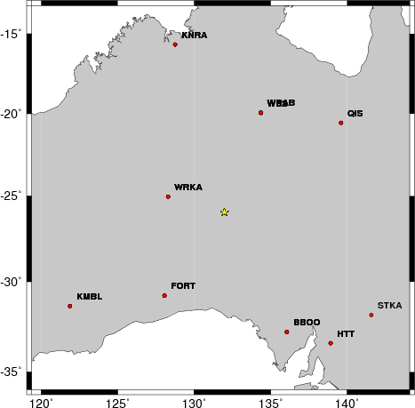
Waveform Inversion

The focal mechanism was determined using broadband seismic waveforms. The location of the event and the and stations used for the waveform inversion are shown in the next figure.

Location of broadband stations used for waveform inversion

The program wvfgrd96 was used with good traces observed at short distance to determine the focal mechanism, depth and seismic moment. This technique requires a high quality signal and well determined velocity model for the Green functions. To the extent that these are the quality data, this type of mechanism should be preferred over the radiation pattern technique which requires the separate step of defining the pressure and tension quadrants and the correct strike.

The observed and predicted traces are filtered using the following gsac commands:

hp c 0.01 n 3
lp c 0.05 n 3

           DEPTH  STK   DIP  RAKE   MW    FIT
WVFGRD96    0.5    95    60    40   5.36 0.7759
WVFGRD96    1.0   100    60    50   5.38 0.7868
WVFGRD96    2.0   280    60    55   5.43 0.7896
WVFGRD96    3.0   115    55    75   5.48 0.7633
WVFGRD96    4.0   115    60    80   5.52 0.7175
WVFGRD96    5.0   300    65    80   5.51 0.6961
WVFGRD96    6.0   300    65    80   5.50 0.6750
WVFGRD96    7.0   300    65    80   5.49 0.6552
WVFGRD96    8.0   295    70    75   5.46 0.6405
WVFGRD96    9.0    75    70   -35   5.44 0.6472
WVFGRD96   10.0   285    75    65   5.45 0.6374
WVFGRD96   11.0    75    70   -35   5.46 0.6477
WVFGRD96   12.0    75    70   -40   5.46 0.6519
WVFGRD96   13.0    80    75   -40   5.45 0.6567
WVFGRD96   14.0    80    75   -40   5.45 0.6602
WVFGRD96   15.0    80    75   -40   5.45 0.6624
WVFGRD96   16.0    80    75   -40   5.46 0.6632
WVFGRD96   17.0    80    75   -40   5.46 0.6634
WVFGRD96   18.0    80    75   -40   5.46 0.6635
WVFGRD96   19.0    85    80   -40   5.46 0.6638
WVFGRD96   20.0   110    85   -60   5.46 0.6603
WVFGRD96   21.0   110    85   -60   5.46 0.6612
WVFGRD96   22.0   110    85   -60   5.47 0.6612
WVFGRD96   23.0   110    85   -60   5.47 0.6614
WVFGRD96   24.0   110    85   -60   5.48 0.6599
WVFGRD96   25.0   110    85   -60   5.48 0.6577
WVFGRD96   26.0   115    85   -60   5.49 0.6561
WVFGRD96   27.0   115    85   -60   5.49 0.6530
WVFGRD96   28.0   115    85   -60   5.49 0.6493
WVFGRD96   29.0   115    85   -60   5.50 0.6461

The best solution is

WVFGRD96    2.0   280    60    55   5.43 0.7896

The mechanism correspond to the best fit is

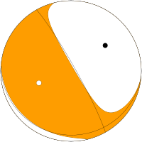
Figure 1. Waveform inversion focal mechanism

The best fit as a function of depth is given in the following figure:

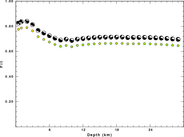
Figure 2. Depth sensitivity for waveform mechanism

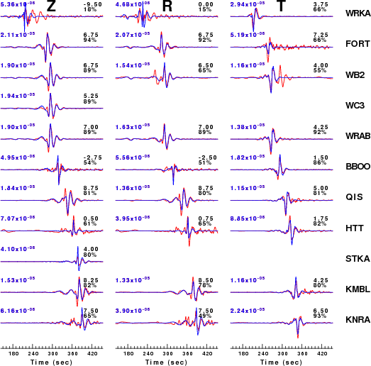
The comparison of the observed and predicted waveforms is given in the next figure. The red traces are the observed and the blue are the predicted. Each observed-predicted component is plotted to the same scale and peak amplitudes are indicated by the numbers to the left of each trace. A pair of numbers is given in black at the right of each predicted traces. The upper number it the time shift required for maximum correlation between the observed and predicted traces. This time shift is required because the synthetics are not computed at exactly the same distance as the observed and because the velocity model used in the predictions may not be perfect. A positive time shift indicates that the prediction is too fast and should be delayed to match the observed trace (shift to the right in this figure). A negative value indicates that the prediction is too slow. The lower number gives the percentage of variance reduction to characterize the individual goodness of fit (100% indicates a perfect fit).

The bandpass filter used in the processing and for the display was

hp c 0.01 n 3
lp c 0.05 n 3

Figure 3. Waveform comparison for selected depth

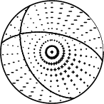
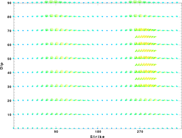
Focal mechanism sensitivity at the preferred depth. The red color indicates a very good fit to thewavefroms. Each solution is plotted as a vector at a given value of strike and dip with the angle of the vector representing the rake angle, measured, with respect to the upward vertical (N) in the figure.

A check on the assumed source location is possible by looking at the time shifts between the observed and predicted traces. The time shifts for waveform matching arise for several reasons:

• The origin time and epicentral distance are incorrect
• The velocity model used for the inversion is incorrect
• The velocity model used to define the P-arrival time is not the same as the velocity model used for the waveform inversion (assuming that the initial trace alignment is based on the P arrival time)

 Time_shift = A + B cos Azimuth + C Sin Azimuth

The time shifts for this inversion lead to the next figure:

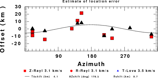
The derived shift in origin time and epicentral coordinates are given at the bottom of the figure.

Discussion

Thanks also to the many seismic network operators whose dedication make this effort possible: University of Alaska, University of Washington, Oregon State University, University of Utah, Montana Bureas of Mines, UC Berkely, Caltech, UC San Diego, Saint Louis University, University of Memphis, Lamont Doherty Earth Observatory, the IRIS stations and the Transportable Array of EarthScope.

Velocity Model

The WUS used for the waveform synthetic seismograms and for the surface wave eigenfunctions and dispersion is as follows:

MODEL.01
CUS Model with Q from simple gamma values
ISOTROPIC
KGS
FLAT EARTH
1-D
CONSTANT VELOCITY
LINE08
LINE09
LINE10
LINE11
  H(KM) VP(KM/S) VS(KM/S) RHO(GM/CC)   QP   QS  ETAP  ETAS  FREFP  FREFS
  1.0000  5.0000  2.8900  2.5000 0.172E-02 0.387E-02 0.00  0.00  1.00  1.00 
  9.0000  6.1000  3.5200  2.7300 0.160E-02 0.363E-02 0.00  0.00  1.00  1.00 
 10.0000  6.4000  3.7000  2.8200 0.149E-02 0.336E-02 0.00  0.00  1.00  1.00 
 20.0000  6.7000  3.8700  2.9020 0.000E-04 0.000E-04 0.00  0.00  1.00  1.00 
  0.0000  8.1500  4.7000  3.3640 0.194E-02 0.431E-02 0.00  0.00  1.00  1.00 

Quality Control

Here we tabulate the reasons for not using certain digital data sets

The following notes are made about station recordings. I processed the traces in the same manner as above, e.g., in the0.01 - 0.05 Hz band use the Sac commands given above.

• AS31 horizontals could not be used because of non-lienar response due to the short epicentral distance.
• The AS31 vertical seems to have a gain that is too large by a factor of 20. This is indicated by the fact that the predicted motion in the waveform plot is significantly larger than the observed motion
• QIS has problems. Either the station location is wrong or the channel information does not fit. Given the station location and compoent orientation, the rotation from ZNE to ZRT gives Rayleigh wave on the T component and the Love wave on the R component. The NEIC location gives an azimuth of 54.0 to the station, while the Geoscience Australia location gives az azimuth of 54.98. Thus the station location in the metadata is OK.
• However, the P-wave first motion is DOWN to the NORTH WEST. If the vertical modtion is OK, then the expected motion is Down to the South West.
• SO IS THERE A METADATA, WIRING OR INSTALLATION PROBLEM?