2012/06/19 10:53:29 -38.244 146.194 9.9 5.20 Australia
USGS Felt map for this earthquake
 USGS/SLU Moment Tensor Solution
 ENS  2012/06/19 10:53:29:0 -38.24  146.19   9.9 5.2 Australia

 Stations used:
   AU.CMSA AU.CNB AU.TOO AU.YNG

 Filtering commands used:
   hp c 0.02 n 3
   lp c 0.04 n 3

 Best Fitting Double Couple
  Mo = 3.13e+23 dyne-cm
  Mw = 4.93
  Z  = 11 km
  Plane   Strike  Dip  Rake
   NP1      225    80    75
   NP2      102    18   146
  Principal Axes:
   Axis    Value   Plunge  Azimuth
    T   3.13e+23     53     117
    N   0.00e+00     15     228
    P  -3.13e+23     33     328

 Moment Tensor: (dyne-cm)
    Component   Value
       Mxx    -1.31e+23
       Mxy     5.16e+22
       Mxz    -1.91e+23
       Myy     2.80e+22
       Myz     2.11e+23
       Mzz     1.03e+23


                     --------------
                 ----------------------
              ----------------------------
             ------   -------------------##
           -------- P ----------------#######
          ---------   --------------##########
         ------------------------##############
        -----------------------#################
        ---------------------###################
       #-------------------######################
       #-----------------########################
       #----------------#########################
       ##-------------#############   ###########
        #-----------############### T ##########
        ##---------################   #########-
         ##------#############################-
          ###---#############################-
           ################################--
             #---########################--
              -------################-----
                 ----------------------
                     --------------


 Global CMT Convention Moment Tensor:
      R          T          P
  1.03e+23  -1.91e+23  -2.11e+23
 -1.91e+23  -1.31e+23  -5.16e+22
 -2.11e+23  -5.16e+22   2.80e+22


Details of the solution is found at

http://www.eas.slu.edu/Earthquake_Center/MECH.NA/20120619105329/index.html
|
      STK = 225
      DIP = 80
     RAKE = 75
       MW = 4.93
       HS = 11.0
The waveform inversion is preferred.
The following compares this source inversion to others
 USGS/SLU Moment Tensor Solution
 ENS  2012/06/19 10:53:29:0 -38.24  146.19   9.9 5.2 Australia

 Stations used:
   AU.CMSA AU.CNB AU.TOO AU.YNG

 Filtering commands used:
   hp c 0.02 n 3
   lp c 0.04 n 3

 Best Fitting Double Couple
  Mo = 3.13e+23 dyne-cm
  Mw = 4.93
  Z  = 11 km
  Plane   Strike  Dip  Rake
   NP1      225    80    75
   NP2      102    18   146
  Principal Axes:
   Axis    Value   Plunge  Azimuth
    T   3.13e+23     53     117
    N   0.00e+00     15     228
    P  -3.13e+23     33     328

 Moment Tensor: (dyne-cm)
    Component   Value
       Mxx    -1.31e+23
       Mxy     5.16e+22
       Mxz    -1.91e+23
       Myy     2.80e+22
       Myz     2.11e+23
       Mzz     1.03e+23


                     --------------
                 ----------------------
              ----------------------------
             ------   -------------------##
           -------- P ----------------#######
          ---------   --------------##########
         ------------------------##############
        -----------------------#################
        ---------------------###################
       #-------------------######################
       #-----------------########################
       #----------------#########################
       ##-------------#############   ###########
        #-----------############### T ##########
        ##---------################   #########-
         ##------#############################-
          ###---#############################-
           ################################--
             #---########################--
              -------################-----
                 ----------------------
                     --------------


 Global CMT Convention Moment Tensor:
      R          T          P
  1.03e+23  -1.91e+23  -2.11e+23
 -1.91e+23  -1.31e+23  -5.16e+22
 -2.11e+23  -5.16e+22   2.80e+22


Details of the solution is found at

http://www.eas.slu.edu/Earthquake_Center/MECH.NA/20120619105329/index.html
|
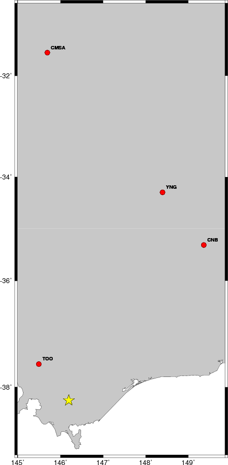
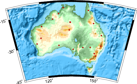
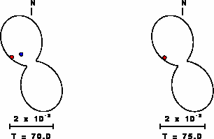
The focal mechanism was determined using broadband seismic waveforms. The location of the event and the and stations used for the waveform inversion are shown in the next figure.
|
|
|
|
The program wvfgrd96 was used with good traces observed at short distance to determine the focal mechanism, depth and seismic moment. This technique requires a high quality signal and well determined velocity model for the Green functions. To the extent that these are the quality data, this type of mechanism should be preferred over the radiation pattern technique which requires the separate step of defining the pressure and tension quadrants and the correct strike.
The observed and predicted traces are filtered using the following gsac commands:
hp c 0.02 n 3
lp c 0.04 n 3
The results of this grid search from 0.5 to 19 km depth are as follow:
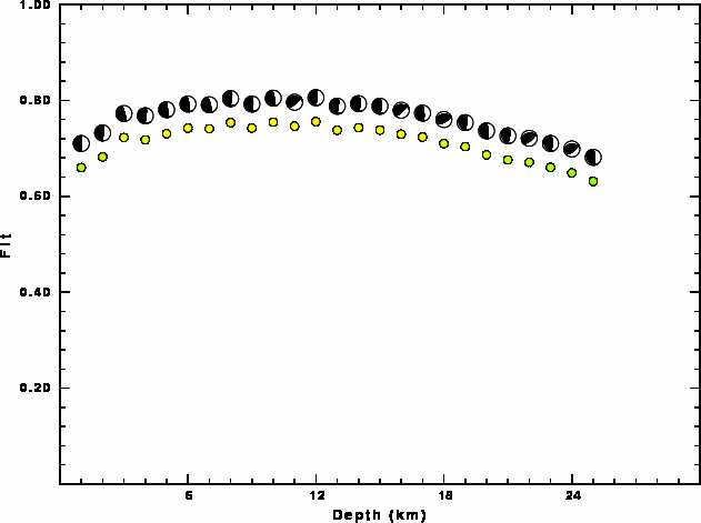
           DEPTH  STK   DIP  RAKE   MW    FIT
WVFGRD96    0.5   250    40    90   4.75 0.6279
WVFGRD96    1.0   250    45    90   4.77 0.6242
WVFGRD96    2.0    20    90   -80   5.13 0.6613
WVFGRD96    3.0    30    90   -80   5.04 0.7349
WVFGRD96    4.0   225    85    80   4.98 0.7989
WVFGRD96    5.0   225    85    80   4.96 0.8369
WVFGRD96    6.0   235    80    80   4.94 0.8587
WVFGRD96    7.0   235    80    80   4.93 0.8909
WVFGRD96    8.0   235    80    80   4.91 0.9020
WVFGRD96    9.0   235    80    80   4.90 0.9092
WVFGRD96   10.0   235    80    80   4.93 0.9150
WVFGRD96   11.0   225    80    75   4.93 0.9153
WVFGRD96   12.0   225    80    75   4.92 0.9115
WVFGRD96   13.0    10    85   -65   5.00 0.9015
WVFGRD96   14.0   225    80    75   4.91 0.8928
WVFGRD96   15.0   200    90    65   4.95 0.8827
WVFGRD96   16.0   200    90    65   4.95 0.8722
WVFGRD96   17.0    10    85   -65   4.99 0.8629
WVFGRD96   18.0     5    80   -65   5.00 0.8497
WVFGRD96   19.0    10    80   -60   4.99 0.8383
WVFGRD96   20.0     5    80   -65   5.03 0.8247
WVFGRD96   21.0     5    80   -65   5.03 0.8089
WVFGRD96   22.0     5    80   -60   5.04 0.7939
WVFGRD96   23.0     5    80   -60   5.04 0.7782
WVFGRD96   24.0     5    80   -60   5.04 0.7621
WVFGRD96   25.0     5    75   -55   5.05 0.7470
WVFGRD96   26.0     5    75   -55   5.05 0.7317
WVFGRD96   27.0     0    70   -55   5.08 0.7167
WVFGRD96   28.0     0    70   -55   5.08 0.7023
WVFGRD96   29.0     0    70   -55   5.08 0.6881
The best solution is
WVFGRD96 11.0 225 80 75 4.93 0.9153
The mechanism correspond to the best fit is
|
|
|
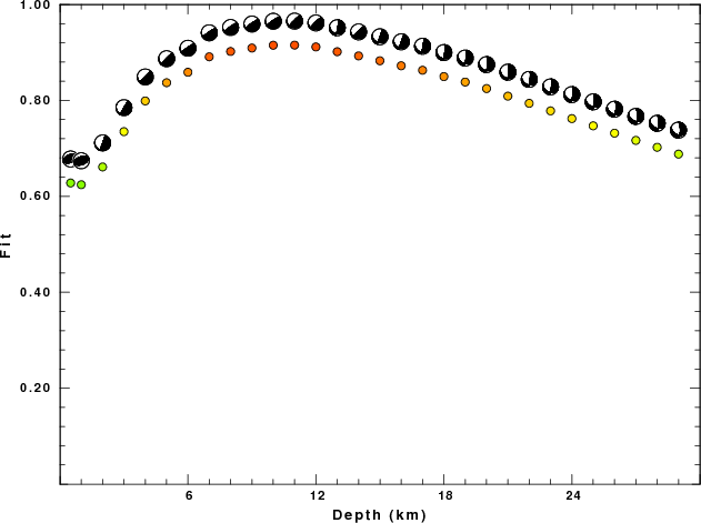
The best fit as a function of depth is given in the following figure:
|
|
|
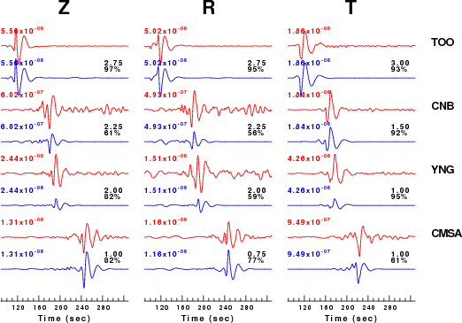
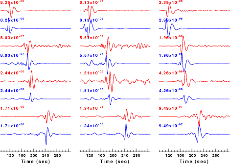
The comparison of the observed and predicted waveforms is given in the next figure. The red traces are the observed and the blue are the predicted. Each observed-predicted component is plotted to the same scale and peak amplitudes are indicated by the numbers to the left of each trace. A pair of numbers is given in black at the right of each predicted traces. The upper number it the time shift required for maximum correlation between the observed and predicted traces. This time shift is required because the synthetics are not computed at exactly the same distance as the observed and because the velocity model used in the predictions may not be perfect. A positive time shift indicates that the prediction is too fast and should be delayed to match the observed trace (shift to the right in this figure). A negative value indicates that the prediction is too slow. The lower number gives the percentage of variance reduction to characterize the individual goodness of fit (100% indicates a perfect fit).
The bandpass filter used in the processing and for the display was
hp c 0.02 n 3
lp c 0.04 n 3
|
|
|
|
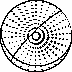
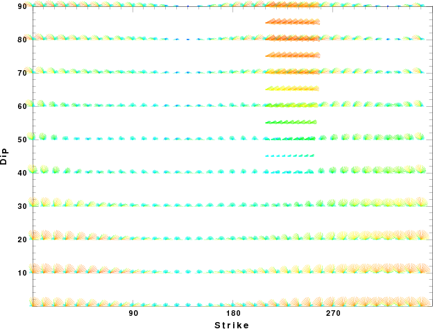
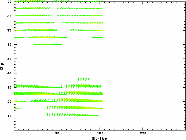
| Focal mechanism sensitivity at the preferred depth. The red color indicates a very good fit to thewavefroms. Each solution is plotted as a vector at a given value of strike and dip with the angle of the vector representing the rake angle, measured, with respect to the upward vertical (N) in the figure. |
A check on the assumed source location is possible by looking at the time shifts between the observed and predicted traces. The time shifts for waveform matching arise for several reasons:
Time_shift = A + B cos Azimuth + C Sin Azimuth
The time shifts for this inversion lead to the next figure:
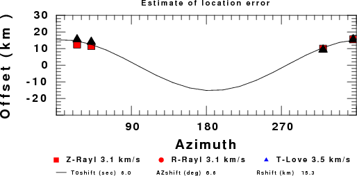
The derived shift in origin time and epicentral coordinates are given at the bottom of the figure.
The following figure shows the stations used in the grid search for the best focal mechanism to fit the surface-wave spectral amplitudes of the Love and Rayleigh waves.
|
|
|
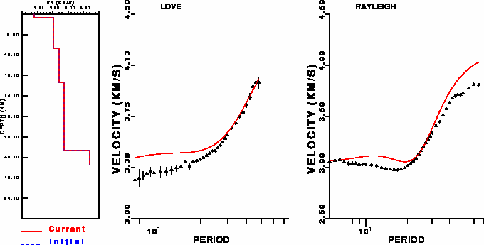
The surface-wave determined focal mechanism is shown here.
  NODAL PLANES


  STK=      50.00
  DIP=      69.99
 RAKE=    -105.00

             OR

  STK=     268.07
  DIP=      24.82
 RAKE=     -54.59


DEPTH = 11.0 km

Mw = 4.98
Best Fit 0.7462 - P-T axis plot gives solutions with FIT greater than FIT90
 |
The P-wave first motion data for focal mechanism studies are as follow:
Sta Az Dist First motion
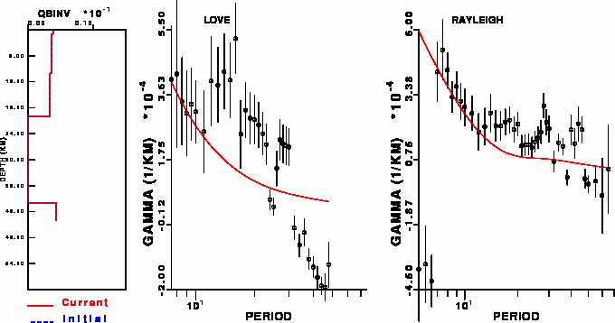
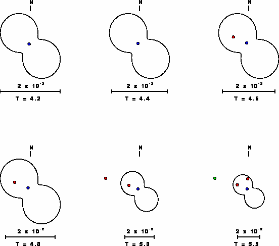
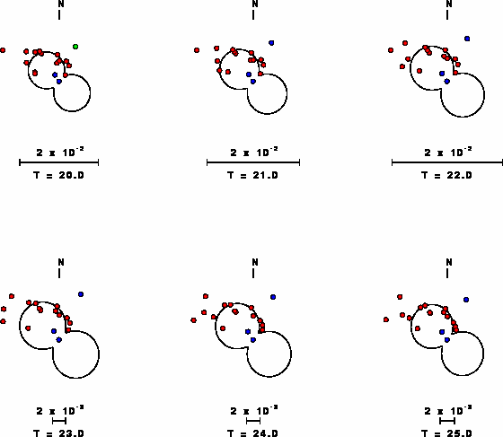
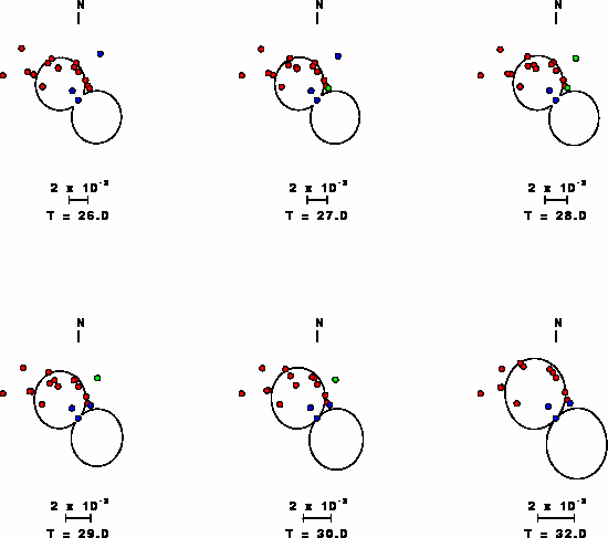
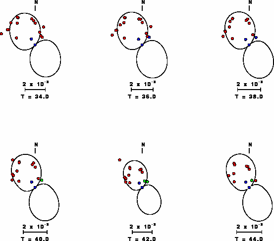
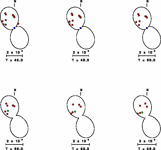
Surface wave analysis was performed using codes from Computer Programs in Seismology, specifically the multiple filter analysis program do_mft and the surface-wave radiation pattern search program srfgrd96.
Digital data were collected, instrument response removed and traces converted
to Z, R an T components. Multiple filter analysis was applied to the Z and T traces to obtain the Rayleigh- and Love-wave spectral amplitudes, respectively.
These were input to the search program which examined all depths between 1 and 25 km
and all possible mechanisms.
|
|
|

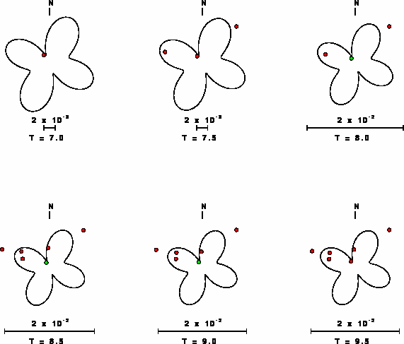
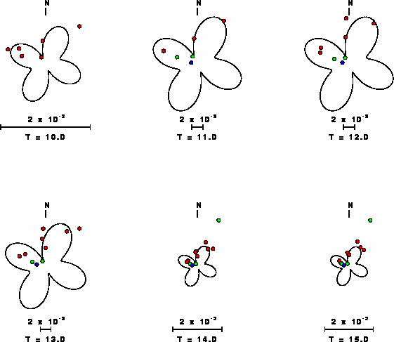
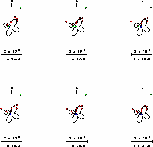
|
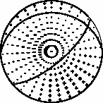
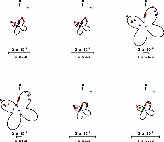
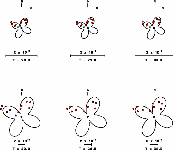
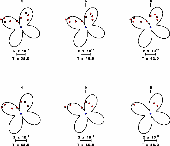
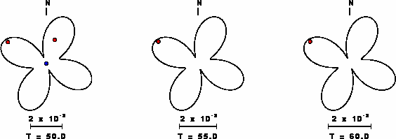
| Pressure-tension axis trends. Since the surface-wave spectra search does not distinguish between P and T axes and since there is a 180 ambiguity in strike, all possible P and T axes are plotted. First motion data and waveforms will be used to select the preferred mechanism. The purpose of this plot is to provide an idea of the possible range of solutions. The P and T-axes for all mechanisms with goodness of fit greater than 0.9 FITMAX (above) are plotted here. |
|
| Focal mechanism sensitivity at the preferred depth. The red color indicates a very good fit to the Love and Rayleigh wave radiation patterns. Each solution is plotted as a vector at a given value of strike and dip with the angle of the vector representing the rake angle, measured, with respect to the upward vertical (N) in the figure. Because of the symmetry of the spectral amplitude rediation patterns, only strikes from 0-180 degrees are sampled. |
The distribution of broadband stations with azimuth and distance is
Listing of broadband stations used
Since the analysis of the surface-wave radiation patterns uses only spectral amplitudes and because the surfave-wave radiation patterns have a 180 degree symmetry, each surface-wave solution consists of four possible focal mechanisms corresponding to the interchange of the P- and T-axes and a roation of the mechanism by 180 degrees. To select one mechanism, P-wave first motion can be used. This was not possible in this case because all the P-wave first motions were emergent ( a feature of the P-wave wave takeoff angle, the station location and the mechanism). The other way to select among the mechanisms is to compute forward synthetics and compare the observed and predicted waveforms.
The fits to the waveforms with the given mechanism are show below:
|
This figure shows the fit to the three components of motion (Z - vertical, R-radial and T - transverse). For each station and component, the observed traces is shown in red and the model predicted trace in blue. The traces represent filtered ground velocity in units of meters/sec (the peak value is printed adjacent to each trace; each pair of traces to plotted to the same scale to emphasize the difference in levels). Both synthetic and observed traces have been filtered using the SAC commands:
hp c 0.02 n 3
lp c 0.04 n 3
|
|
Should the national backbone of the USGS Advanced National Seismic System (ANSS) be implemented with an interstation separation of 300 km, it is very likely that an earthquake such as this would have been recorded at distances on the order of 100-200 km. This means that the closest station would have information on source depth and mechanism that was lacking here.
Dr. Harley Benz, USGS, provided the USGS USNSN digital data. The digital data used in this study were provided by Natural Resources Canada through their AUTODRM site http://www.seismo.nrcan.gc.ca/nwfa/autodrm/autodrm_req_e.php, and IRIS using their BUD interface.
Thanks also to the many seismic network operators whose dedication make this effort possible: University of Alaska, University of Washington, Oregon State University, University of Utah, Montana Bureas of Mines, UC Berkely, Caltech, UC San Diego, Saint L ouis University, Universityof Memphis, Lamont Doehrty Earth Observatory, Boston College, the Iris stations and the Transportable Array of EarthScope.
The CUS model was used for the waveform synthetic seismograms and for the surface wave eigenfunctions and dispersion is as follows:
MODEL.01
CUS Model with Q from simple gamma values
ISOTROPIC
KGS
FLAT EARTH
1-D
CONSTANT VELOCITY
LINE08
LINE09
LINE10
LINE11
  H(KM) VP(KM/S) VS(KM/S) RHO(GM/CC)   QP   QS  ETAP  ETAS  FREFP  FREFS
  1.0000  5.0000  2.8900  2.5000 0.172E-02 0.387E-02 0.00  0.00  1.00  1.00
  9.0000  6.1000  3.5200  2.7300 0.160E-02 0.363E-02 0.00  0.00  1.00  1.00
 10.0000  6.4000  3.7000  2.8200 0.149E-02 0.336E-02 0.00  0.00  1.00  1.00
 20.0000  6.7000  3.8700  2.9020 0.000E-04 0.000E-04 0.00  0.00  1.00  1.00
  0.0000  8.1500  4.7000  3.3640 0.194E-02 0.431E-02 0.00  0.00  1.00  1.00
Here we tabulate the reasons for not using certain digital data sets
The following stations did not have a valid response files:
DATE=Mon Jun 25 02:33:01 CDT 2012