#!/bin/sh
#####
# clean up
#####
rm -f *.png
rm -f *.PLT
cat > SCM.mod << EOF create the velocity model
MODEL.01
Simple crustal model
ISOTROPIC
KGS
FLAT EARTH
1-D
CONSTANT VELOCITY
LINE08
LINE09
LINE10
LINE11
H(KM) VP(KM/S) VS(KM/S) RHO(GM/CC) QP QS ETAP ETAS FREFP FREFS
40.0000 6.0000 3.5500 2.8000 0.00 0.00 0.00 0.00 1.00 1.00
0.0000 8.0000 4.7000 3.3000 0.00 0.00 0.00 0.00 1.00 1.00
EOF
cat > dfile << EOF create the file that
10.0 0.25 256 0 0 gives distance, dt, npts, t0 vred
20.0 0.25 256 0 0
30.0 0.25 256 0 0
40.0 0.25 256 0 0
50.0 0.25 256 0 0
60.0 0.25 256 0 0
70.0 0.25 256 0 0
80.0 0.25 256 0 0
90.0 0.25 256 0 0
100.0 0.25 256 0 0
110.0 0.25 256 0 0
120.0 0.25 256 0 0
130.0 0.25 256 0 0
140.0 0.25 256 0 0
150.0 0.25 256 0 0
160.0 0.25 256 0 0
170.0 0.25 256 0 0
180.0 0.25 256 0 0
190.0 0.25 256 0 0
200.0 0.25 256 0 0
EOF
#####
# we will make synthetics for the receiver above and below the interface
#####
mkdir INTERFACE_ALL_TOP
hprep96 -M SCM.mod -d dfile -ALL -HS 21 -HR 20 -TH -BH Create the control for the program hspec96. Since the
model file has a reference layer of 40 km, the source is placed 19 km above the
interfce, and the receiver is 20 km above the interface.
hspec96 -SD
Only consider waves leaving the source in a downward direction.
Because of the source position, the synthetics will not have a direct wave
Now put in the source time function, convert to Sac files and place in a subdirectory
hpulse96 -V -p -l 1 | \
(cd INTERFACE_ALL_TOP ; f96tosac -G )
# make plots
gsac << EOF
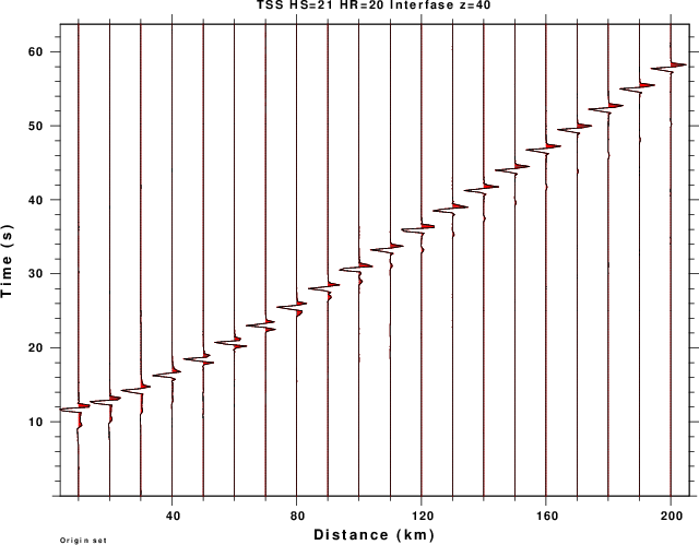
r INTERFACE_ALL_TOP/*TSS
title on location top size small text "TSS HS=21 HR=20 Interfase z=40"
bg plt
prs amp 0.25 color 2 shd neg
shade the negative amplitudes of the trace in the color red
mv PRS001.PLT TOP_TSS.PLT
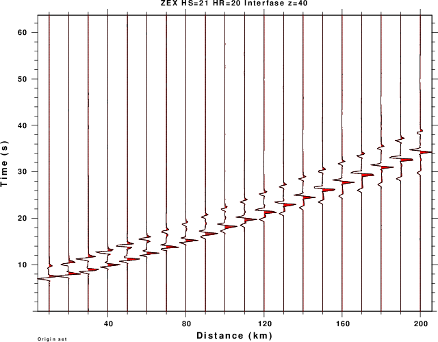
r INTERFACE_ALL_TOP/*ZEX
title on location top size small text "ZEX HS=21 HR=20 Interfase z=40"
bg plt
color red
prs amp 0.25
mv PRS002.PLT TOP_ZEX.PLT
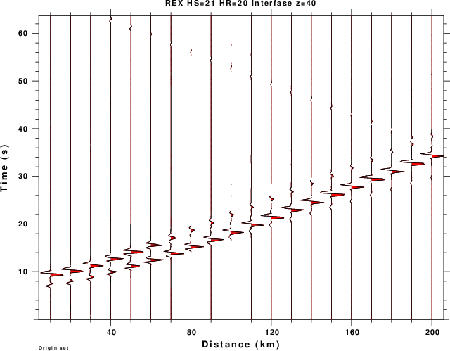
r INTERFACE_ALL_TOP/*REX
title on location top size small text "REX HS=21 HR=20 Interfase z=40"
bg plt
color blue
prs amp 0.25
mv PRS003.PLT TOP_REX.PLT
q
EOF
mkdir INTERFACE_ALL_BOT
hprep96 -M SCM.mod -d dfile -ALL -HS 21 -HR 60 -TH -BH
hspec96 -SD
hpulse96 -V -p -l 1 | \
(cd INTERFACE_ALL_BOT ; f96tosac -G )
gsac << EOF
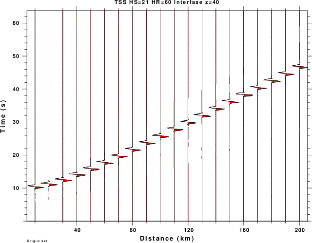
r INTERFACE_ALL_BOT/*TSS
title on location top size small text "TSS HS=21 HR=60 Interfase z=40"
bg plt
prs amp 0.25 color 2 shd neg
mv PRS001.PLT BOT_TSS.PLT
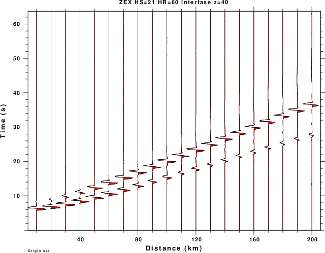
r INTERFACE_ALL_BOT/*ZEX
title on location top size small text "ZEX HS=21 HR=60 Interfase z=40"
bg plt
color red
prs amp 0.25
mv PRS002.PLT BOT_ZEX.PLT
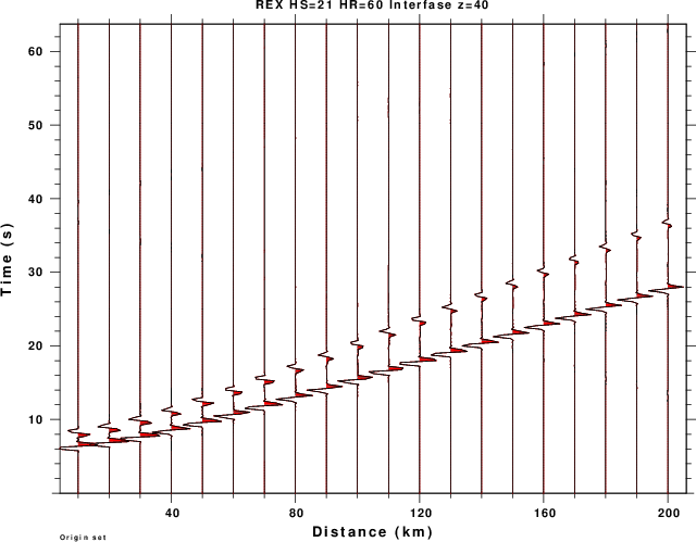
r INTERFACE_ALL_BOT/*REX
title on location top size small text "REX HS=21 HR=60 Interfase z=40"
bg plt
color blue
prs amp 0.25
mv PRS003.PLT BOT_REX.PLT
q
EOF
Each external plot in a gsac execution has a unique identifier. Thus three PRS calls create PRS001.PLT PRS002.PLT PRS003.PLT
#####
# some representative traces
#####
gsac << EOF
color list red blue
fileid name
r INTERFACE_ALL_BOT/0160*[ZR]EX
title on location top size small text "Z (red) R(blue) 160 km HS=21 HR=60 Interfase z=40"
bg plt
p overly on
r INTERFACE_ALL_TOP/0160*[ZR]EX
title on location TOP size small text "Z (red) R(blue) 160 km HS=21 HR=20 Interfase z=40"
p overly on
q
EOF
Here the plot calls create P001.PLT and P002.PLT
mv P001.PLT BOT_160.PLT
mv P002.PLT TOP_160.PLT
for i in ???_???.PLT
do
B=`basename $i .PLT`
plotnps -F7 -W10 -EPS -K < $i > t.eps
convert -trim t.eps -background white -alpha remove $B.png
done
#####
# clean up
#####
rm -f hspec96.???
rm -f PRS*.CTL
rm -f t.eps
rm -f dfile
rm -f *.PLT
|
| TOP_TSS.png | Transverse component reflections from strike slip source |
| TOP_REX.png | Radial component (away from source) from expansion source |
| TOP_ZEX.png | Vertical component (away from source) from expansion source |
| TOP_160.png | Overlay of vertical (up) and radial (away) components from EX source at 160 km |
| BOT_TSS.png | Transverse component reflections from strike slip source |
| BOT_REX.png | Radial component (away from source) from expansion source |
| BOT_ZEX.png | Vertical component (away from source) from expansion source |
| BOT_160.png | Overlay of vertical (up) and radial (away) components from EX source at 160 km |
|
|
|
|
|
|
|
|
It is interesting to overlay the traces to look at particle motion
to determine the nature of the wave.
Exercise