This exercise shows how to estimate phase velocities beneath a
network from a teleseismic surface wave signal observed by all
stations. The concept is to assume that the Earth structure
beneath the seismic network is uniform and that the incident
wavefront from the distance source follows a great circle path so
that the signal arrivals at two stations at the same distance at the
same time. The analysis essentially projects the observed waveforms
onto a linear array in the center of the network and the p-omega
stacking is then performed.
In order to do this, data
processing must account for the requirements of the stacking program
sacpom96 (which is called by the GUI do_pom). First the
traces must be of the same length, second, the traces must be
resampled to a lower sample rate for efficiency in the stacking (to
make the fast Fourier transforms faster because the number of points
is smaller), the fundamental mode surface wave must be isolated for a
good stack (using the GUI do_mft which calls sacmft96
to determine the group velocity dispersion and then sacmat96
to isolate the fundamental mode. Finally do_pom cat be run.
The data set used for this tutorial is Sac.tgz
Download this file and unpack is using the command
gunzip -c Sac.tgz | tar xvf -
This will create a subdirectory Sac and place the waveform forms in
that directory.
Since these SAC files are coming from an Intel
machine, you must make sure that the files are in the correct byte
order by performing the commands
cd Sac
for i in *Sac
do
        saccvt -I < $i > tmp
        mv tmp $i
done
Now you can work with the data
You must put the event information into the trace headers. you can do this using gsac as follows (I assume that you are in the Sac directory)
gsac
GSAC - Computer Programs in Seismology [V1.1.21 13 SEP 2007]
       Copyright 2004, 2005, 2006, 2007 R. B. Herrmann
GSAC> r *Z.Sac
CHUBHZ.Sac HDBBHZ.Sac KANBHZ.Sac KWJBHZ.Sac PUSBHZ.Sac SEOBHZ.Sac SOGBHZ.Sac TAGBHZ.Sac TEJBHZ.Sac TJNBHZ.Sac ULLBHZ.Sac
GSAC> ch evla 6.898 evlo 126.579 evdp 33
GSAC> ch ocal 2001 01 01 06 57 01 172
GSAC> wh
GSAC> quit
Since I assume that the trace headers
already had the station
latitude and longitude fields set (STLA and STLO), the trace headers
will now have the DIST, GCARC, AZ and BAZ fields set.
If I
have GMT installed, I can do the following from within gsac
GSAC> r *Z.Sac
CHUBHZ.Sac HDBBHZ.Sac KANBHZ.Sac KWJBHZ.Sac PUSBHZ.Sac SEOBHZ.Sac SOGBHZ.Sac TAGBHZ.Sac TEJBHZ.Sac TJNBHZ.Sac ULLBHZ.Sac
GSAC> map r on
r on
Execute using the command: sh map.sh
GSAC> sh map.sh
sh map.sh
pscoast: Working on block #   301
pscoast: Adding Borders...
GSAC>
The file map.eps is created and you can view it using gs, display or other PostScript viewers. You will see the following: map.png
The next step is to view the traces and to examining the header for the sample interval since the analysis requires that all traces have the same sample interval, DELTA, and the same number of points. Note that these traces are the original digital data. The instrument response has not been removed. Normally deconvolution is necessary, but if the instruments have identical response, then deconvolution is not necessary. Such is the case for these data.
GSAC> r *Z.Sac
CHUBHZ.Sac HDBBHZ.Sac KANBHZ.Sac KWJBHZ.Sac PUSBHZ.Sac SEOBHZ.Sac SOGBHZ.Sac TAGBHZ.Sac TEJBHZ.Sac TJNBHZ.Sac ULLBHZ.Sac
GSAC> sort up dist
Sorting on DIST in ascending order
GSAC> lh delta npts
SOGBHZ.Sac (6):
NPTS 6601 DELTA 0.2
KWJBHZ.Sac (3):
NPTS 6601 DELTA 0.2
PUSBHZ.Sac (4):
NPTS 6601 DELTA 0.2
HDBBHZ.Sac (1):
NPTS 80001 DELTA 0.05
TAGBHZ.Sac (7):
NPTS 6601 DELTA 0.2
TEJBHZ.Sac (8):
NPTS 6601 DELTA 0.2
TJNBHZ.Sac (9):
NPTS 80001 DELTA 0.05
SEOBHZ.Sac (5):
NPTS 6601 DELTA 0.2
ULLBHZ.Sac (10):
NPTS 6601 DELTA 0.2
KANBHZ.Sac (2):
NPTS 6601 DELTA 0.2
CHUBHZ.Sac (0):
NPTS 6601 DELTA 0.2
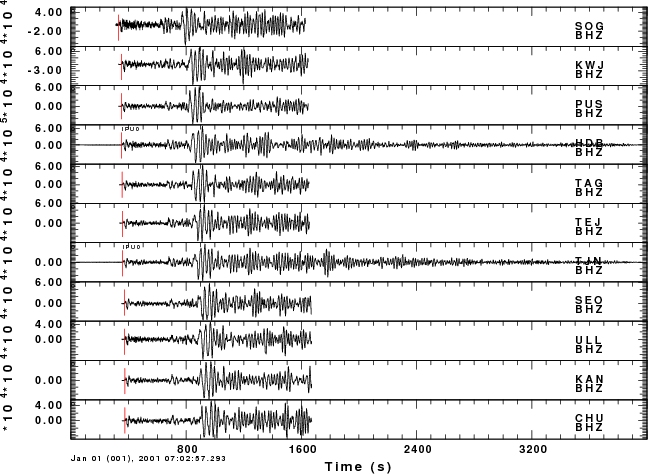
GSAC> p
You will not the different sampling intervals and the different
number of points, The command "p" plots the
traces:
We use this figure to design the cut to isolate the signal and then we resample to a DELTA=0.5 sec with the following commands
GSAC> r *Z.Sac
CHUBHZ.Sac HDBBHZ.Sac KANBHZ.Sac KWJBHZ.Sac PUSBHZ.Sac SEOBHZ.Sac SOGBHZ.Sac TAGBHZ.Sac TEJBHZ.Sac TJNBHZ.Sac ULLBHZ.Sac
GSAC> rtr
GSAC> w
CHUBHZ.Sac HDBBHZ.Sac KANBHZ.Sac KWJBHZ.Sac PUSBHZ.Sac SEOBHZ.Sac SOGBHZ.Sac TAGBHZ.Sac TEJBHZ.Sac TJNBHZ.Sac ULLBHZ.Sac
GSAC> synchronize o
GSAC> wh
GSAC> cuterr fillz
GSAC> cut o 300 o 1800
cut o 300 o 1800
O 300.000000 O 1800.000000
GSAC> r *Z.Sac
CHUBHZ.Sac HDBBHZ.Sac KANBHZ.Sac KWJBHZ.Sac PUSBHZ.Sac SEOBHZ.Sac SOGBHZ.Sac TAGBHZ.Sac TEJBHZ.Sac TJNBHZ.Sac ULLBHZ.Sac
GSAC> lp c 1 n 2 p 2
LP: corner fc 1.000000  npoles 2 pass 2 Butterworth
GSAC> interpolate delta 0.5
delta 0.5
GSAC> cd ..
Current directory is /home/rbh/PROGRAMS.310t/PROGRAMS.330.fixups/TUTORIAL/POMEGA
GSAC> mkdir GOOD
mkdir GOOD
GSAC> cd GOOD
Current directory is /home/rbh/PROGRAMS.310t/PROGRAMS.330.fixups/TUTORIAL/POMEGA/GOOD
GSAC> w
CHUBHZ.Sac HDBBHZ.Sac KANBHZ.Sac KWJBHZ.Sac PUSBHZ.Sac SEOBHZ.Sac SOGBHZ.Sac TAGBHZ.Sac TEJBHZ.Sac TJNBHZ.Sac ULLBHZ.Sac
GSAC> pwd
pwd
/home/rbh/PROGRAMS.310t/PROGRAMS.330.fixups/TUTORIAL/POMEGA/GOOD
GSAC>
This is what was done. Read the traces and remove and linear
trend, and then write the traces out. Reset the time reference as the
origin time using synchronize. Then plot the trace and see
that the surface wave is in the window 300 to 1800 seconds after the
origin time. Reread and add zeros to the beginning and end of traces
if necessary. The low pass filter with a zero phase filter at 1.0 Hz,
and finally interpolate to a sample of 0.5 seconds.
Since
I do not want to destroy the original data, I create a new directory
parallel to the Sac directory with the SHELL command cd ..
followed by mkdir GOOD. We then move from the current
directory to that new directory and write the traces there. If
I read these new traces in I see the following with a lh npts
delta
GSAC> lh npts delta
SOGBHZ.Sac (6):
         NPTS                 3001        DELTA                  0.5
KWJBHZ.Sac (3):
         NPTS                 3001        DELTA                  0.5
PUSBHZ.Sac (4):
         NPTS                 3001        DELTA                  0.5
HDBBHZ.Sac (1):
         NPTS                 3001        DELTA                  0.5
and the plot
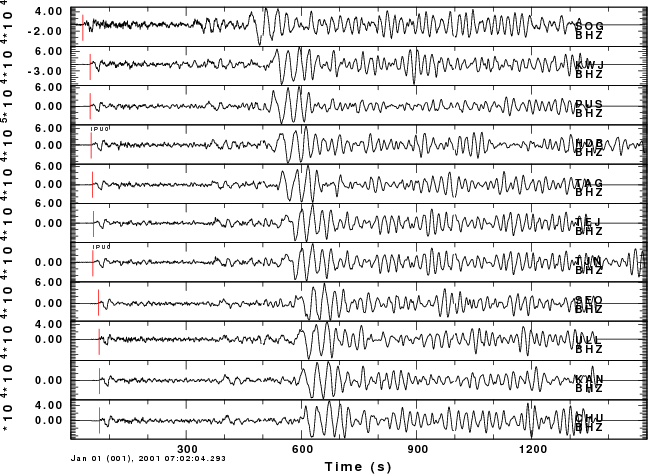
In the GOOD directory, issue the command
do_mft *Z.Sac
Then select one trace, TAG, for example, and run do_mft and select
the dispersion curve. Since this is a large earthquake, I instruct
do_mft to look at periods between 4 and 300 seconds. I select
dispersion between 20 and 200 seconds:
Now hit the Match button. on the next page, select Match and then Fund for the fundamental mode. Then select No and then Quit
If you look at the
console, you will see the following command when do_mft started
the phase match filter program sacmat96
/home/rbh/PROGRAMS.310t/PROGRAMS.330/bin/sacmat96 -F TAGBHZ.Sac -D disp.d -AUTO
We will use this as a prototype to phase match all traces through a
SHELL script. The reason for doing it this way is that there is no
certainty that all traces will have the
same range of dispersion
periods for and individual phase match filter. So create the
script DOIT. make it executable and run in the GOOD directory
which also has the disp.d dispersion file. Here is DOIT
#!/bin/sh
for i in *Z.Sac
do
sacmat96 -F $i -D disp.d -AUTO
done
No after you execute it you see the following files in the GOOD directory
CHUBHZ.Sac   disp.out     KANBHZ.Sacr  mft96.ctl   PUSBHZ.Sac   SOGBHZ.Sac   TEJBHZ.Sac   ULLBHZ.Sac
CHUBHZ.Sacr  DOIT*        KANBHZ.Sacs  mft96.disp  PUSBHZ.Sacr  SOGBHZ.Sacr  TEJBHZ.Sacr  ULLBHZ.Sacr
CHUBHZ.Sacs  HDBBHZ.Sac   KWJBHZ.Sac   mft96.ods   PUSBHZ.Sacs  SOGBHZ.Sacs  TEJBHZ.Sacs  ULLBHZ.Sacs
disp.d       HDBBHZ.Sacr  KWJBHZ.Sacr  MFT96.PLT   SEOBHZ.Sac   TAGBHZ.Sac   TJNBHZ.Sac
disp.dp      HDBBHZ.Sacs  KWJBHZ.Sacs  P001.PLT    SEOBHZ.Sacr  TAGBHZ.Sacr  TJNBHZ.Sacr
disp.dv      KANBHZ.Sac   MFT96CMP     P002.eps    SEOBHZ.Sacs  TAGBHZ.Sacs  TJNBHZ.Sacs
The files ending in .Sacs are the isolated
fundamental
mode. The sum of the traces .Sacs and .Sacr
gives the original trace. If you read the *Z.Sacs and plot
under gsac you will see
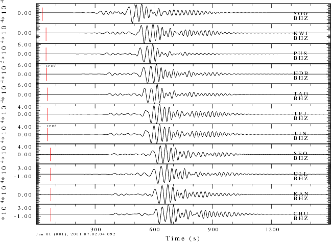
Notice
how the body waves and scatter surface waves have been removed.
In the directory GOOD run the command
do_pom *Z.Sacs
Hit the commands SelectAll, Do Pom on page 1,
then select 4 and 200 for the period limits, Shade
on, Type Rayleigh, Nray 250, and Length 4
followed by Do Pom on page 2, and wait. You will then be
presented with a editing screen to select the phase velocities. Then
save the dispersion by clicking on Exit and then Yes.
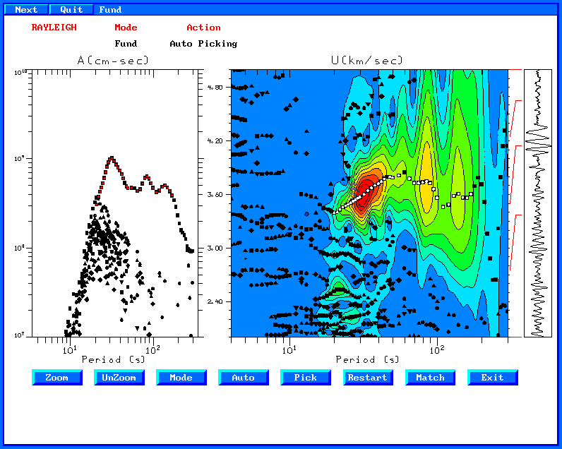
The output dispersion is in the file disp.d which is in a surf96
dispersion format. The dispersion plot with selected dispersion
is
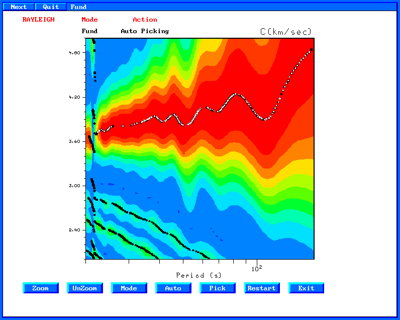
Here
are some of the dispersion points
SURF96 R C X  0       86.23     4.21690     0.24200    10.7102
SURF96 R C X  0       80.31     4.22890     0.19760    10.7777
SURF96 R C X  0       84.45     4.22890     0.22800    10.7340
SURF96 R C X  0       81.92     4.24100     0.20980    10.7623
SURF96 R C X  0         128     4.28920     0.49920    10.4922
SURF96 R C X  0         130     4.33730     0.52780    10.4752
SURF96 R C X  0       132.1     4.38550     0.55780    10.4582
SURF96 R C X  0       134.3     4.42170     0.58610    10.4410
SURF96 R C X  0       136.5     4.46990     0.61910    10.4236
SURF96 R C X  0       138.9     4.51810     0.65350    10.4064
SURF96 R C X  0       141.2     4.55420     0.68550    10.3900
You will notice that the dispersion is not perfectly uniform. This
may be due to the fact that the path from the earthquake to each
station may have slightly different propagation which violated our
assumption of circular wavefronts.
Perform this
operation for a numebr of earthquakes, from different regions, so
that you get a good sampling of the dispersion.
Last changed March 11,
2009