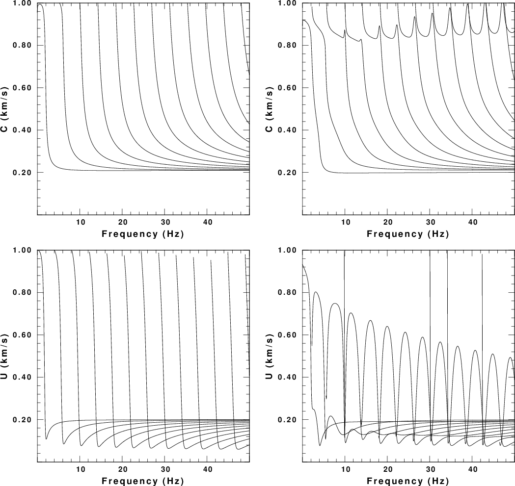
Fig. 1. Dispersion curves for the test model. The first row gives phase velocity and the second gives group velocity. The left column is for Love waves and the right is for Rayleigh waves.
The measurement of H/V is documented in several places:
This tutorial will focus on the generation of synthetic Z, N and E waveforms in Sac format.
gunzip -c HVNOISE.tgz | tar xf -This procedure creates a directory strucutre and puts the processing files there:
	HVNOISE.dist/
	HVNOISE.dist/DOITHVHF
	HVNOISE.dist/DOSPECRAT
	HVNOISE.dist/Models/
	HVNOISE.dist/Models/
	HVNOISE.dist/Models/soilm2.mod
	HVNOISE.dist/Models/soil.mod
	HVNOISE.dist/Models/CUS.mod
For the example here, we consider the velocity model HVNOISE.dist/Models/soilm2.mod. The dispersion curves for this model are given Figure 1. The fundamental and higher modes are plotted. The odd behavior for the Rayleigh wave pahse velocities near the velocity of about 0.8 km/s is due to the use of a causal Q operator and the low Q of the upper layer of the model. The group velocities are for infinite Q. The group velocities indicate that there could be arrivals propagating as slow as 80 m/s. (0.08 km/sec).
Fig. 1. Dispersion curves for the test model. The first row gives phase velocity and the second gives group velocity. The left column is for Love waves and the right is for Rayleigh waves. |
Figure 2 displays the Rayleigh wave ellipticity and the factor AR /sqrt(k). Although the synthetic noise in the example will have Love and Rayleigh wave contributions, the measured H/V ratio should be affected by the Rayleigh wave ellipticity. This the ellipticity plot may assist in the interpretation of the measured H/V ratio. The other quantity plotted is related to the excitation of the Rayleigh wave. For a vertical source at the surface, the vertical component displacement will be proportional to
AR 1/sqrt(kr) UZ UZ
I have dropped the phase term. Assuming that the UZ eigenfunction is 1.0 at the surface, then the spectral amplitude of a mode is
proportional to AR /sqrt(k)
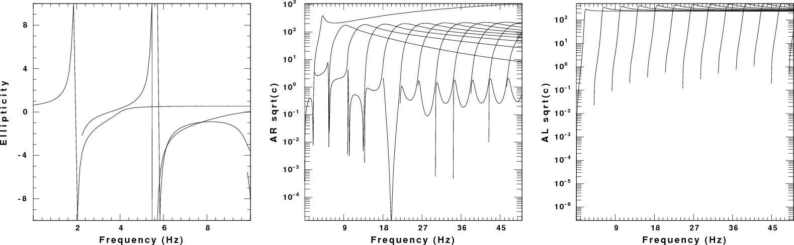 Fig. 2. Left: Rayleigh wave ellipticity for this model. Center: Rayleigh wave amplitude term. Right; Love wave amplitude term. |
From these two figures we can conclude that the fundamental mode dominates the spectral amplitude up to a frequency of about 9 Hz, and thus the fundamental mode ellipticity at 2 Hz should be what controls the empirical H/V ratio. Because the excitation of the Love wave is comparable to that of the fundamental model rayleigh wave, we might say that the observed H/V ratio is dominated by the Rayleigh wave ellipticity near 2 Hz. Note that the important factor may be the frequency at which the H/V ratio is a maximum rather than the actual peak value of the ratio.
As set up, the script DOITHVHF ultimately creates 900 seconds of 3-component noise as the sac files E.stk, N.stk and Z.stk. The user can then process these time series to determine the H/V ratio using their own or other routines. The script DOSPECRAT uses these series to create CSV files of the amplitude spectra through the gsac command outcsv.
The initial part of DOSPECRAT sets up the parameters for the simulation. This part is as follows:
	#!/bin/bash

	#####
	#    create a noise data set by generating synthetic
	#    motions from randomly distributed point forces
	#    applied at the surface
	#
	#    To reflect real data we create individual segments
	#    define the power spectra and finally the ratio tp get H/V
	#
	#    This script is designed for high frequency
	#    motions for local site studies
	#####

	#####
	#    Velocity model
	#####
	VMOD="Models/soilm2.mod"
	#####
	#    for surface wave synthetics
	#####
	NMODE=100		The maximum number of modes to include depends on the velocity model

	#####
	#    noise sources:  These occur in the region
	#    -XMAX <= x <= XMAX
	#    -YMAX <= y <= YMAX
	#    except about a region DMIN about the receiver
	#####
	DELTA=0.01      # sample interval in seconds

	DMIN=0.005      # exclude sources within DMIN km of receiver     These may be adequate for a local survey at high frequency
	XMAX=1.000      # define source region
	YMAX=1.000

	#####
	#    define the receiver coordinate
	#    XR,YR
	#####
	XR=0.0
	YR=0.0

	#####
	TMAX=900        # The sac file will 0 to TMAX seconds long
	#
	NSRC=10000      # number of random sources			This is an extensive run
	                # these will occur at intervals of TMAX/NSRC seconds


	################### do not change after here #####################
The next part of the script defines some functions. The details of the functions are not given in this description.
	function getvmodextreme () {
	#####
	#    examine the velocity model to determine the
	#    minimum and maximum shear velocities which
	#    will be used for the noise sampling
	#
	#   the following are returned globally:
	#   VMIN - minimum S velocity in the model
	#   VMAX - maximum S velocity in the model
	#####
	}

	function getsrc()
	{
	#####
	#    get random coordinates in the region
	#    -XMAX ≤ x ≤ XMAX
	#    -YMAX ≤ y ≤ YMAX
	#
	#   the following are returned globally:
	#   (XS,YS) - source coordinates in km
	#   (EVAL,EVLO) - source coordinate in geocentrc coordinates
	#           - for simplicity the receivers are assumed to be
	#           - near (0,0) so that te conversion from km to degree
	#           - does is essentially cartesian
	#####
	}

	function getforce()
	{
	#####
	#    get the components for the force to be applied at the surface
	#    the following are returned globally:
	#    FN - force component in north direction
	#    FE - force component in east  direction
	#    FD - force component in down  direction
	#
	#####
	}
The last part of the script performs the simulation:
	##### everything below here does the synthetic of the noise #####

	#####
	#    clean up previouse run
	#####
	rm -f ??????.stk

	#####
	#    get the extreme values of the S velocity from the model
	#####
	getvmodextreme
	echo VMIN=$VMIN VMAX=$VMAX

	#####
	#    first generate the eigenfunctions so that the
	#    synthetics can be made
	#    The time window must be long enough to encompass the
	#    arrivals at the fastest and slowest velocities
	#####
	NPT=`echo $XMAX $YMAX $VMIN $VMAX $DELTA | awk \
		'{ DIST=sqrt($1*$1 + $2*$2) ; TWIN=(DIST/$3 ) ; print int(TWIN/$5)}' `
	DIST=`echo $XMAX $YMAX | awk '{print sqrt($1*$1 + $2*$2)}' `
	echo DIST $DIST XMAX $XMAX YMAX $YMAX
	cat > ddfile << EOF
	${DIST} ${DELTA} ${NPT} 0.0 0.0
	EOF
	sprep96  -M ${VMOD} -HS 0 -HR 0 -L -R -NMOD ${NMODE} -d ddfile
	sdisp96
	sregn96
	slegn96
	FNYQ=`echo $DELTA | awk '{print 0.5/$1}' `

	#####
	#    make plot of the dispersion of the form
	#    LC RC
	#    LU RU
	#####
	rm -fr S?EGN?.PLT
	rm -f DISP.PLT
	sdpegn96 -L -C  -XLIN -YLIN -X0 2.0 -Y0 8 -XLEN 6 -YLEN 6 -YMIN 0 -YMAX ${VMAX} -XMIN 0.0 -XMAX ${FNYQ}
	sdpegn96 -L -U  -XLIN -YLIN -X0 2.0 -Y0 1 -XLEN 6 -YLEN 6 -YMIN 0 -YMAX ${VMAX} -XMIN 0.0 -XMAX ${FNYQ}
	sdpegn96 -R -C  -XLIN -YLIN -X0 9.5 -Y0 8 -XLEN 6 -YLEN 6 -YMIN 0 -YMAX ${VMAX} -XMIN 0.0 -XMAX ${FNYQ}
	sdpegn96 -R -U  -XLIN -YLIN -X0 9.5 -Y0 1 -XLEN 6 -YLEN 6 -YMIN 0 -YMAX ${VMAX} -XMIN 0.0 -XMAX ${FNYQ}
	cat S?EGN?.PLT > DISP.PLT

	#####
	#    now make the synthetics
	#    for each subsource
	#        get source coordinates
	#        get force orientation
	#        make synthetic
	#        use gsac to apply the force
	#        open the synthetic using cut o 0 o TMAX
	#        save
	#    then stack the subsources
	#####
	count=1
	while [ $count -lt ${NSRC} ]
	do
		SRC=`echo $count | awk '{printf "%6.6d", $1}' `
		getsrc
	#	echo $EVLA $EVLO $XS $YS
		getforce
	#	echo $FN $FE $FD
		DIST=`echo $XS $YS $XR $YR | awk '{ DX=$1-$3; DY=$2-$4;print sqrt(DX*DX + DY*DY)}'`
		#####
		#   Y = north
		#   X = east
		#####
		AZ=`echo $XS $YS $XR $YR | awk '{DX=$3-$1;DY=$4-$2;print atan2(DX,DY)*180/3.1514927 }' `
		BAZ=`echo $XR $YR $XS $YS| awk '{DX=$3-$1;DY=$4-$2;print atan2(DX,DY)*180/3.1514927 }' `
		TSHIFT=`echo $SRC $NSRC $TMAX | awk '{WIN=$3/$2; print ($1 -1.) *  WIN}'`
		######
		# check to see that DIST > DMIN
		#####
		ANS=`echo $DIST $DMIN | awk '{ if ( $1 >= $2 ) print "YES" ; else print "NO" }' `
	        if [ $ANS = "YES" ]
		then

	cat > dfile << EOF
	${DIST} ${DELTA} ${NPT} 0.0 0.0
	EOF
		#####
		#   clean up from previous run
		#####
		rm -f *.[ZRT][DSEHV][[DSXF]
		spulse96 -V -p -l 2 -d dfile -EXF | f96tosac -G
		F=`ls *.ZVF`
		B=`basename $F .ZVF`

	gsac << EOF
	mt to ZNE AZ ${AZ} BAZ ${BAZ} FN $FN FE $FE FD $FD FILE $B
	shift F ${TSHIFT}
	w
	q
	EOF
		mv T.Z ${SRC}.Z
		mv T.N ${SRC}.N
		mv T.E ${SRC}.E
		count=`expr $count + 1 `
		fi
	done

	#####
	#    make the final stack
	#####
	gsac << EOF
	cut o o ${TMAX}
	r ??????.E
	stack relative
	ch kcmpnm E
	w E.stk

	r ??????.N
	stack relative
	ch kcmpnm N
	w N.stk

	r ??????.Z
	stack relative
	ch kcmpnm Z
	w Z.stk

	q
	EOF
The script assumes that the three-component noise data set is 900 seconds long. It then processes succeeding 50 sec windows of the simulated nosie by removing a mean trend, applying a Hanning window, computing the spectra, saving the amplitude spectrum, smoothing it using a 21 point mean smoother, and then saving the result as a CSV file (which can be read by Excel).
Then awk is used to form the ratio of the geometric mean of horizontal spectra to the vertical spectra for each window. When this is done an arithmetic average of the ratios is formed.
Finally genplt is used to make a plot of the individual estimates of the H/V ratio. The result is shown in the next figure:
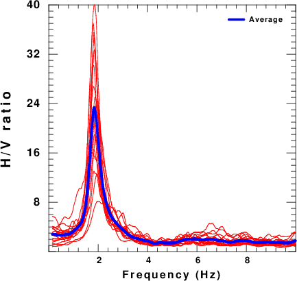 Fig. 3. Plot of individual H/V ratios (red) and the average ratio |
This is a forward simulation. This tutorial does not consider te inverse problem of how the H/V ratio can be use to define structure.