Estimating Source Time Function Using Empirical/Synthetic Green Function

Estimating Source Time Function Using Empirical/Synthetic Green's Function

Introduction

For most seismologists, large earthquakes are interesting not only because of the effects caused but also because of their size. One unresolved question is "what causes an earthquake to be big?" This may be answered in the future through a better understanding of what actually occurs during a large earthquake in terms of which parts of the fault move, how much do they move, and how fast. Methodologies exist to perform a finite fault inversion, which entails using the information from seismographic recordings to image the rupture process on the fault plane. Such analysis requires computaion. Detail fault rupture analysis has implications for estimating the shaking effects near an earthquake by characterizing the rupture plane and the rupture direction.

In the context of hazard estimation, response time is important. The question arises whether it is possible to quickly determine if the rupture process was simple or | complex. One way to make a simple determination is try to determine an average source time function for the earthquake.

Installation

The file DECON.tgz contains the directory structure and processing scripts to perform the deconvolution.
After downloading, execute the following command to unpack the distribution:

gunzip -c DECON.tgz | tar xvf -

which will unpack the following files and directories:

DECON/PROTO.EMP/
DECON/PROTO.EMP/DOITEMP
DECON/PROTO.GRN/
DECON/PROTO.GRN/DOMKSYN
DECON/PROTO.GRN/DOITGRN

These scripts use the programs saclhdr, saciterd and gsac. To do the graphics we need the GraphicsMagick gm (the ImageMagick convert can be used by slightly modify the script) and GMT for the map displays.

The scripts are discussed in the following links:

Empirical Green's Function Processing:
- Discussion of DOITEMP
Synthetic Green's Function Processing:
- Discussion of DOITGRN
- Discussion of DOMKSYN

Execution

Assume that we have already prepared teleseismic data by removing the instrument response, rotating traces, and QC'ing waveforms and that they are placed on the system in the order used for telemseismic source inversion or for using teleseismic for quality control. We will set up the processing using empirical and synthetic Green's functions.

Let directory for the deconvolved, rotated, QC'd wavforms for the large earthquake be

    /home/rbh/PROGRAMS.310t/MOMENT_TENSOR/MECH.TEL/20070815234057/DAT.TEL

and let the directory for the small earthquake used as an empirical Green's function be

    /home/rbh/PROGRAMS.310t/MOMENT_TENSOR/MECH.TEL/20070818025235/DAT.TEL

Now go to the DECON directory created by unpacking the DECON.tgz file and create two new directories:

mkdir 20070818025235.EMP
mkdir 20070818025235.GRN

Now copy the prototype files into the appropriate directory, e.g.,

    cp PROTO.EMP/* 20070818025235.EMP
    cp PROTO.GRN/* 20070818025235.GRN

Finally edit the files in these two directories as follow:

Edit the 20070818025235.EMP/DOITEMP to change the lines

	DIRBIG=path_to_big_event_waveform_directory
	DIRSMALL=path_to_small_event_waveform_directory

	DIRBIG=/home/rbh/PROGRAMS.310t/MOMENT_TENSOR/MECH.TEL/20070815234057/DAT.TEL
	DIRSMALL=/home/rbh/PROGRAMS.310t/MOMENT_TENSOR/MECH.TEL/20070818025235/DAT.TEL

Edit the 20070818025235.GRN/DOITGRN to change the line

	DIRBIG=path_to_big_event_waveform_directory

	DIRBIG=/home/rbh/PROGRAMS.310t/MOMENT_TENSOR/MECH.TEL/20070815234057/DAT.TEL

Also edit the mechanism and source depth lines to use the values expected for the big earthquake:

	STK=171
	DIP=55
	RAKE=112
	HS=30
	MW=5.0

You are now ready to run the codes:

For the empirical Green's function technique

	
	cd 20070818025235.EMP
	DOITEMP

For the synthetic Green's function technique

	cd 20070818025235.GRN
	DOITGRN

Example and Testing

Peru earthquake of August 15, 2007.

This Mw = 8.0 earthquake occurred at 23:40:57.890 UT, had a depth of 39 km, latitude and longitude of -13.39 and -76.60, respectively. We will attempt to define the source time function by comparing this to the Mw=6.0 aftershock on
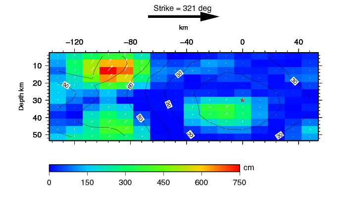
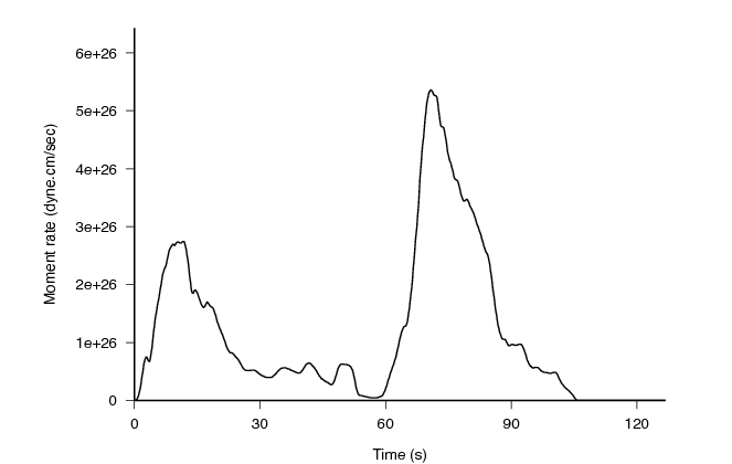
August 18 at 02:52:35 and to synthetic seismograms for a typical mechanism for the region. Fortunately this earthquake was studied by Gavin Hayes of the USGS. Gavin derived a finite fault solution and an averaged source time function.
His finite fault solution and fault averaged (?) moment release is givne in the two figures:

Empirical Green's function deconvolution

For this event we edit the DOITEMP script in the PERU.EMP directory do define the directories containing the waveforms for the main event and the event used as an empirical Green's function:

DIRBIG=/home/rbh/PROGRAMS.310t/MOMENT_TENSOR/MECH.TEL/20070815234057/DAT.TEL
DIRSMALL=/home/rbh/PROGRAMS.310t/MOMENT_TENSOR/MECH.TEL/20070818025235/DAT.TEL

We then execute the script DOITTEMP. The individual station deconvolutions are given in the directory DECONDIR.
In addition several image files are created:
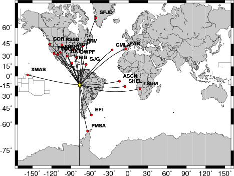
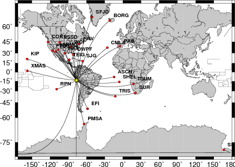
HZ.0.5.map.png - A map of stations whose traces were used with ALP=0.5
HZ.1.0.map.png - A map of stations whose traces were used with ALP=1.0
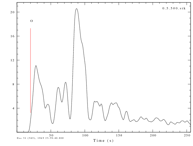
Zdecon.0.5.gif - an azimuthal record section of the individual deconvolutions for ALP=0.5
Zdecon.1.0.gif - an azimuthal record section for ALP=1.0

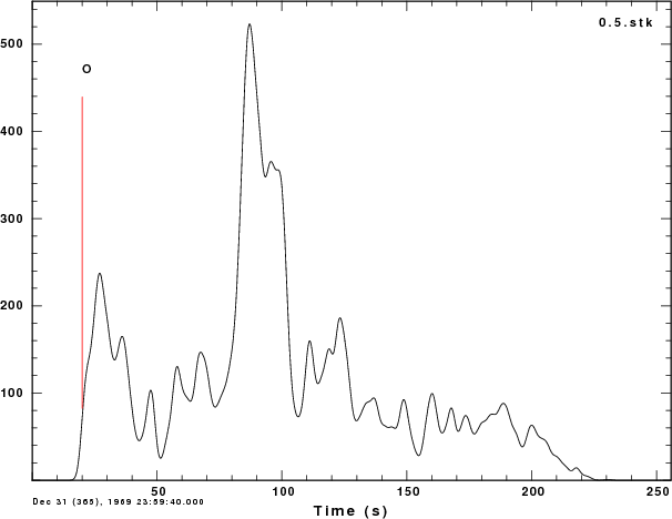
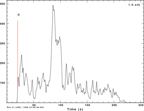
In addition I ran the following gsac commands to get an average of the deconvolutions:

for ALP in 0.5 1.0 
do
gsac << EOF
r DECONDIR/*.${ALP}.decon
stack norm on
w ${ALP}.stk
r ${ALP}.stk
filedid name
bg plt
plotnps -F7 -W10 -EPS -K < P001.PLT  > t.eps
echo using the GraphicsMagick package to convert from eps to png
gm convert -trim t.eps ${ALP}.stk.png
q
EOF
done

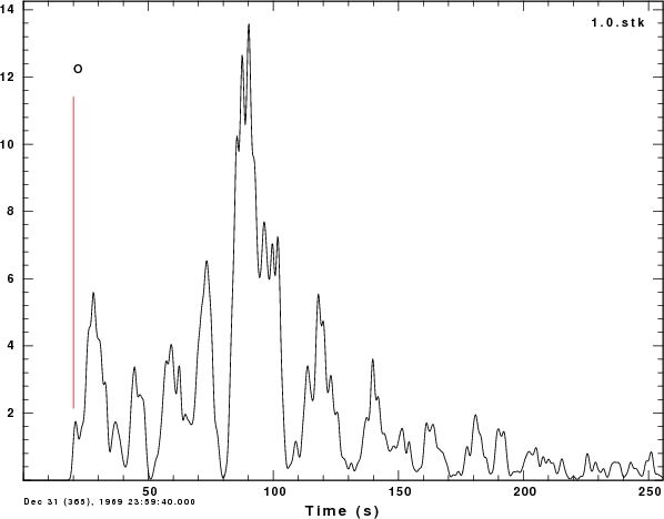
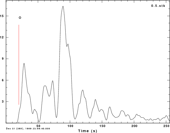
Here are the images:

ALP=0.5	ALP=1.0

We note some similarities between the stacked deconvolutions and the average time function from the finite fault simulation. The effect of using ALP=1.0 is to incorporate higher frequency detail into the estimation. The record sections plotted with azimuth are scaled according to the largest amplitude of all of the deconvolutions. Although the azimuthal sampling is not uniform, there are larger, more compressed waveforms in the direction of rupture progression (141 degrees) than in the opposite direction (321 degrees). This agrees with the more detailed finite fault simulation in which the rupture propagates up dip and in the direction of 141 degrees.

The next test is to compare the results of using 100 versus 500 bumps in the deconvolution procedure for ALP=0.5:

-N 100 -ALP 0.5	-N 500 -ALP 0.5

A feature of using 500 bumps is the increased area under the curve. The sense of an initial event followed 60 seconds later by a larger pulse carries through.

Synthetic Green's function deconvolution

To use synthetics for the small event, we copy the two scripts in PROTO.GRN to PERU.GRN. We then edit the DOITGRN script to provide the location of the seismograms for the main event and the typical mechanism for the region:

DIRBIG=/home/rbh/PROGRAMS.310t/MOMENT_TENSOR/MECH.TEL/20070815234057/DAT.TEL

#####
#       define the mechanism and depth for the synthetics
#       These values can be obtained from the regional
#       averages of mechanisms using the new code
#       STK = strike
#       DIP = dip
#       RAKE = rake
#       HS = sourrce depth in km
#       MW = this is the reference MW, in theory the zero frequency
#       level of the derived source time function is the moment ratio
#       of the two events, e.g., a ratio of 1000 corresponds to a
#       delta Mw of 2.0, so if thw reference Mw=5 then the big event has Mw=7!
#####
STK=171
DIP=55
RAKE=112
HS=30
MW=5.0

We get the average source parameters by running the new USGS code EarthquakeParams.jar through the command line

java -jar EarthquakeParams.jar -radial -13/-76.6/3 -d 0/60 -cn -mt

The output of this command is in the file mtformat.out, the first 15 lines of this file are

Composite Mechanism
Strike  Dip   Rake  
  171    55    112  

MT Format
Radial Search Center Coordinates:    -13.00, -76.60
Radial Search Distance (in deg):       3.0

                        E P I C E N T E R   |          MOMENT      |           M O M E N T    T E N S O R 
     DATE    TIME (UTC)   LAT      LONG  SRC|DEPTH     VAL  EX HALF|SRC  EX         C O M P O N E N T S  
  YR  MO DA HR MN SEC     deg      deg      |  km  Mw       Nm DUR |     Nm  MRR   MTT   MFF   MRT   MRF   MTF 
---------------------------------------------------------------------------------------------------------------
 1976 05 15 21:55:58.50 -11.640  -74.480 MLI| 33.0 6.7 1.7  19  5.7|GCMT 19  0.78 -0.05 -0.73 -0.31  1.41  0.27
 1977 03 08 13:08:56.30 -11.960  -74.200 MLI| 41.0 5.5 2.6  17  2.4|GCMT 17  0.93  0.02 -0.95 -1.32  0.45  2.13
 1980 06 15 23:47:15.00 -15.520  -75.240 MLI| 26.0 5.8 6.2  17  3.0|GCMT 17  2.74  0.73 -3.46 -0.24 -4.97  1.97

the procedure of this script is to use hudson96 to make synthetics for an Mw=5 earthquake. We will look at the deconvolutions for ALP=0.5 and 1.0 again as above.
We will also examine the effect of the assumed source depth on the dseconvolutions:

-N 100 -ALP 0.5	-N 100 -ALP 1.0

In this case we have more azimuths than for the empirical technique since we do not have to worry about the S/Nfor the small event. However we may be affected by instrument response problems which divide out in the empirical technique. We may conclude rupture in the opposite direction from this presentation.

There is more similarity to Gavin's time function, perhaps because both use synthetics.

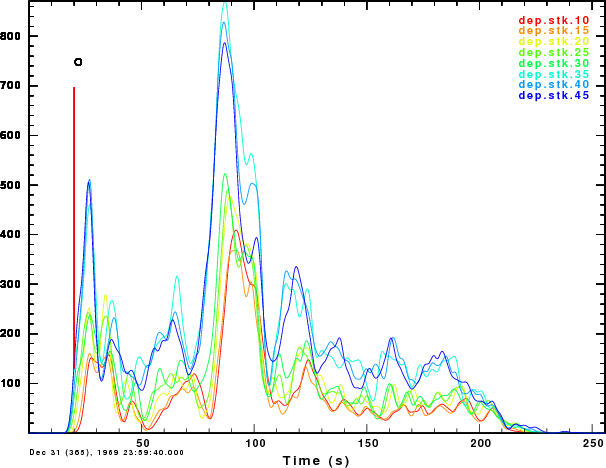
The next test if to consider the sensitivity to the assumed source depth. We consider source depths of 10, 15, 20, 25, 30, 35, 40 and 45 km in the AK135D model.
The figure shows that the double pulse feature is common to all, but that the amplitudes of the two main pulses is affected by sthe assumed source depth, and henc the corresponding moment ratio of the mainshock to the Green's function, since the area under and trace is proporational to the moment ratio.

There is signiicant sensitivity in the deconvolved source pulse to the assumed source depth for the Green's function used to make the predicted motion. This would imply different moment ratios.
Some of the sensitivity may be due to the variation in material properties with depth, with the P velocity increasing from about 6 km/s near the surface to about 8 km/s beneath the Moho wile the density might increase from 2700 to 3300 kg/m^3. Since the teeleseismic amplitude is proportional to Mo/(rho Vp Vp Vp) for the P wave, the teleseismic amplitude for the small Green's event would be decreased by a actor of roughly 2.9, which is what we see in the figure. This simple analysis ignores any of the effects of the depth phases.

Last changed August 14, 2009