Layer3

the purpose of this is to show how ray parameter filtering is applied using cpusle96 and then to discuss the implication.

Everything is run as in the Layer1 example, except that the there are additional options applied to cpulse96, e.g.,

cpulse96 -V -p -l 4 -EXF -DELAY 10 -PMIN 0.08 -PMAX 0.10  | f96tosac -B

Now consider the following plots

CRAY96.PLT

Note that since the input to cseis96 did not change, the same rays were computed.

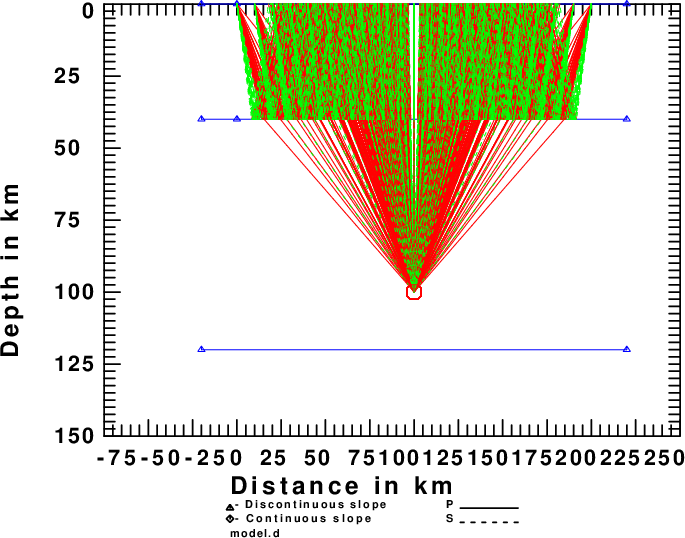
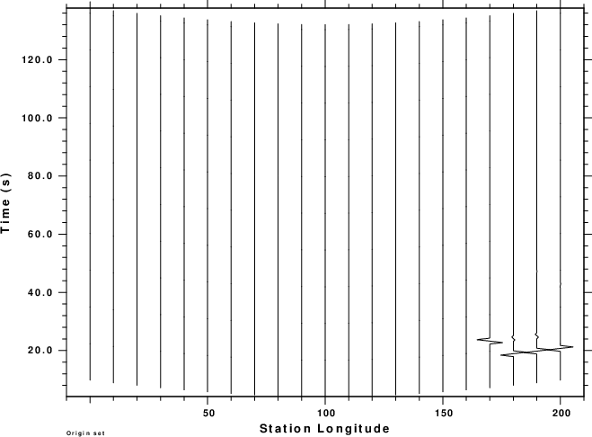
There are two significant differences compared to the Layer1 example. This can be seen in the record sections

ZEX.PLT

REX.PLT

As expected the choice of a positive values for the ray parameter limits did filter reduce the number of rays to make the seismograms. However the synthetics do not look much like those from the Layer1 discussion. By examining the output file cseis96.amp, one sees that many different ray parameters make up the synthetic at 200 km, but only a few of these are in the desired range.

This emphasizes the need to better approximate an indicent plane wave.

Plane wave

To investigate both the ray parameter filtering and also the improvement of the plane-wave approximation, the source position was changed to be deeper and also farther away from the array to give the desired ray parameters. The command sequence is now

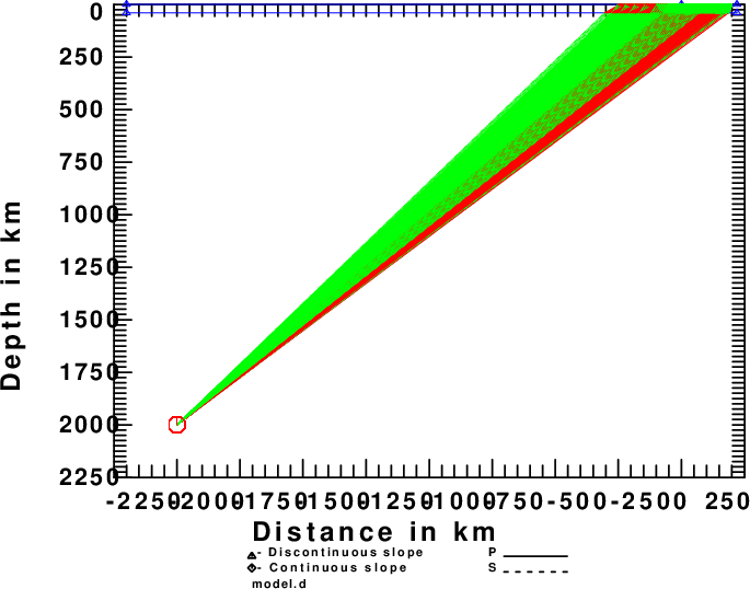
cprep96 -M model.d -d dfile -HS 2000 -XS -2000 -HR 0 -DOALL  -DOCONV
cseis96 -R > cseis96.out
cpulse96 -V -p -l 4 -EXF -DELAY 10 -PMIN 0.08 -PMAX 0.10  | f96tosac -B
cray96 -XMIN -2100 -XMAX 250 -ZMIN 0 -ZMAX 2100

The command line for cprep96 has repositioned the source. The command line for cpulse applies the phase velocity filter. Finally the plot limits forcray96 are changed because of the new source position.

The plots are

CRAY96.PLT

and

ZEX.PLT

REX.PLT

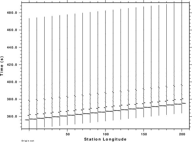It is interesting now that arrivals of all of the receivers are similar. They only differ because of the moveout of the incoming signal across the array. Since the first time sample is delay seconds before the first arrival, an overlay of all traces relative to their beginning would show little difference [GSAC: plot relative overlay on].

Summary

This exercise has shown ray parameter filtering and also the need for a deep source to model plane waves. The horizontal position of that source is determined by trial and error.