The tests demonstrate that the rspec96 gives the
same results as the hspec96 code for the following
media: all liquid layers, all solid layers, a sequence of
liquid layers above solid layers and a sequence of solid layers
above liquid ones.
To test the more difficult solid/liquid/solid problem, rspec96 is run with the solid/liquid/solid model and hspec96 is run with the liquid layer approximated as one with the same P-velocity but with a small, but non-zero S-velocity. It is found that the Z component Green's functions, e.g., ZDD, ZDS, ZSS, ZEX, ZVF and ZHF, are identical throughout the medium. Surprisingly the radial Green's functions, RDD, RDS, RSS, REX, RVF, and RHF agree in the solid layers and also in many of the liquid layers if the very slow S-wave arrival moves away from the initial signal. Because the S-wave velocity is so slow in the approximate medium, the hspec96 results differ from those from rspec96 only near the solid-liquid boundary.
As a result it seems that hspec96 and hspec96p
could be further modified by doing the following:
a) if the medium is fluid/solid/fluid or solid/fluid/solid, etc., set the S-wave velocity for the fluid to be very small. ThenAdmittedly this is a hack, but could useful.
b) run the code but also apply filter for a receiver in fluid of -RPUP -RPDN to filter out the S-wave in the pseudo-fluid.
gunzip -c RSPEC.tgz | tar xf -
cd RSPEC
ls
You will see the directories S, T, SW, WS, and W. In each directory there is a shell script named DOFINAL. Execute those.
The codes rspec96 and rspec96p were tested with isotropic and completely fluid models. The results agreed with those of hspec96 and hspec96p. The critical test is a model consisting of a solid - fluid - solid layer sequence.
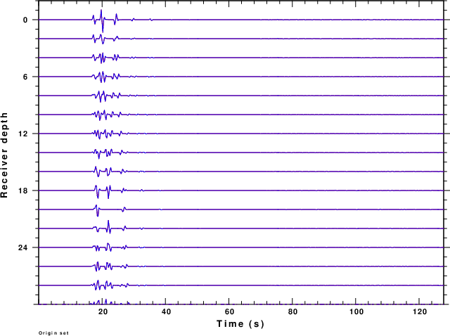
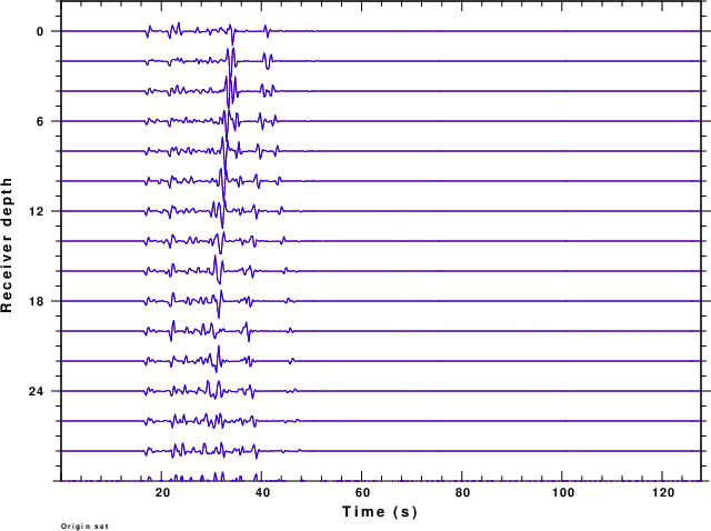
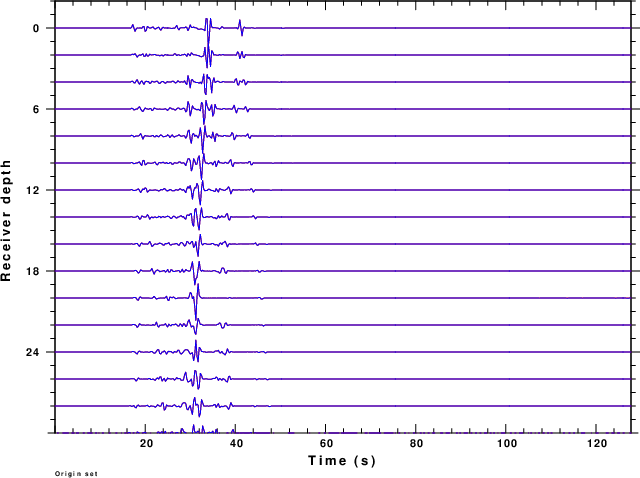
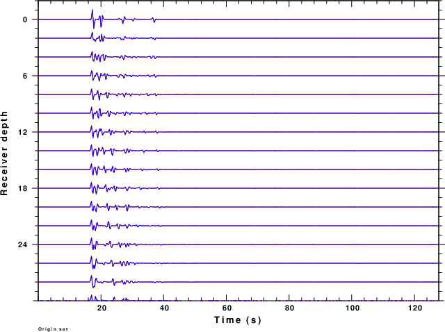
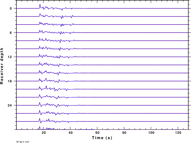
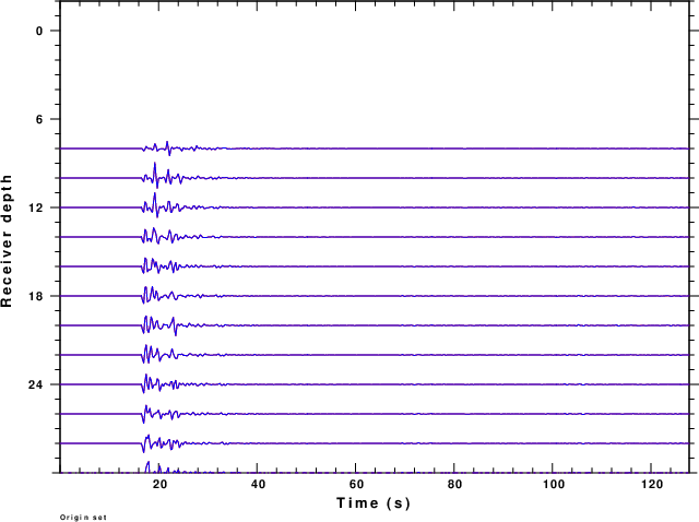
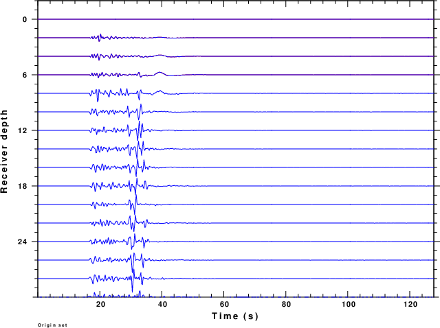
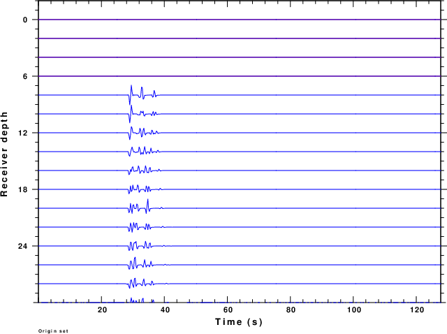
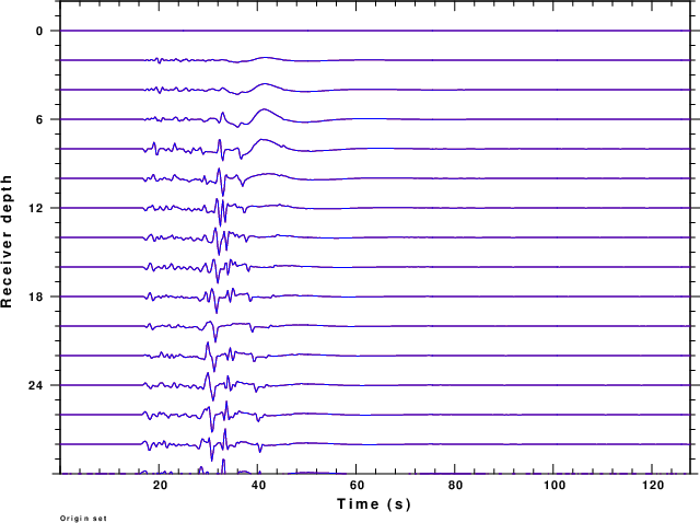
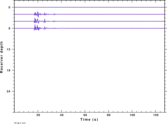
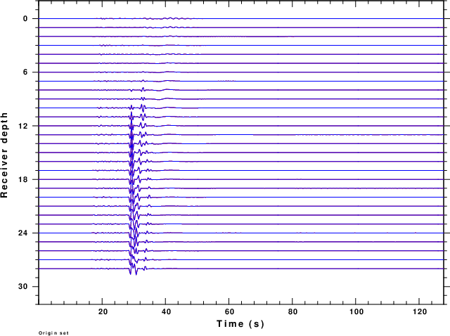
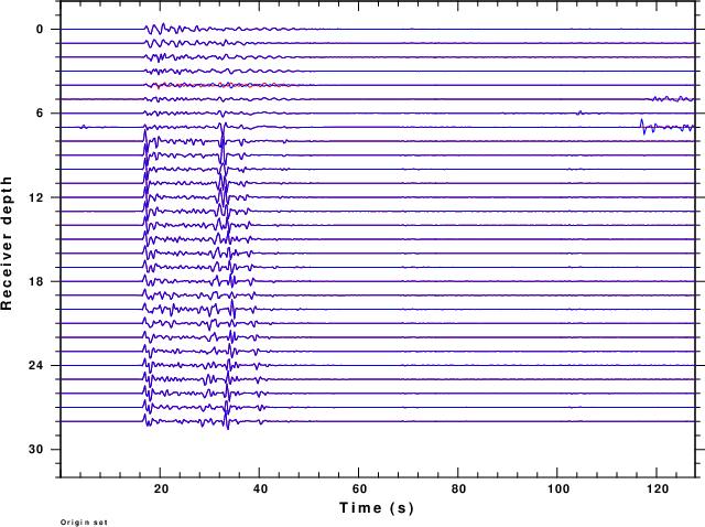
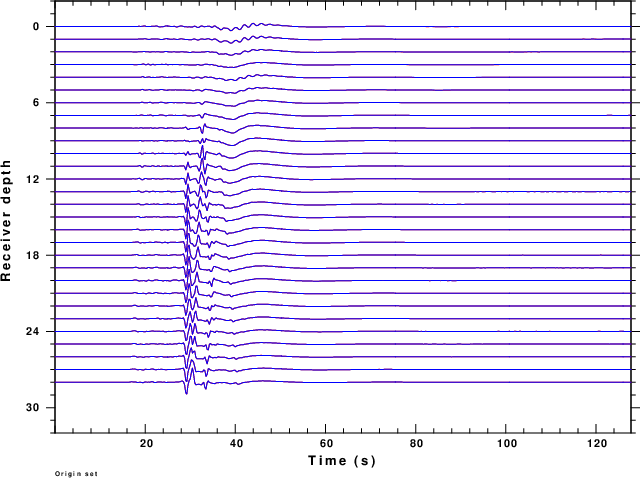
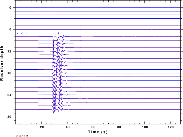
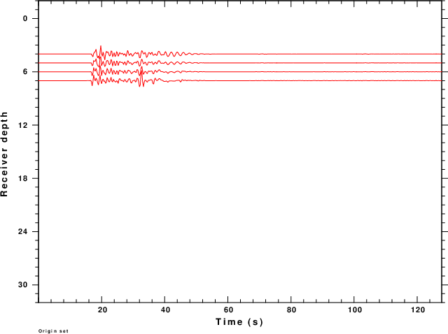
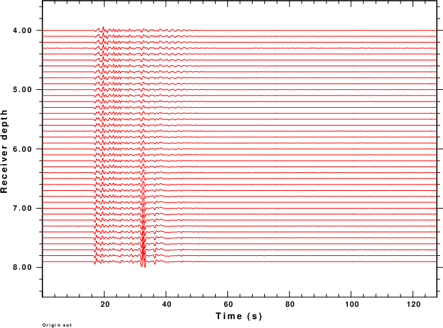
  H(KM) VP(KM/S) VS(KM/S) RHO(GM/CC)   QP   QS  ETAP  ETAS  FREFP  FREFS
  4.0000  6.0000  0.0000  2.7000 0 0 0 0 1 1
  4.0000  6.0000  0.0000  2.7000 0 0 0 0 1 1
  7.0000  6.0000  0.0000  2.7000 0 0 0 0 1 1
 26.0000  6.0000  0.0000  2.7000 0 0 0 0 1 1
   .0000  8.0000  0.0000  3.3000 0 0 0 0 1 1
For this model only the ZEX, REX and PEX Green's functions are created. The source is at a depth of 20 km and the receiver depths vary from the surface to 30 km. The rspec96 and hspec96 Green's functions are plotted in red and blue, respectively. The plots are a true amplitude plot, meaning that the relative amplitudes between rceiver depths is preserved. Click on the links to see the comparison.
The display shows only subtle differences between the results of the two methods.
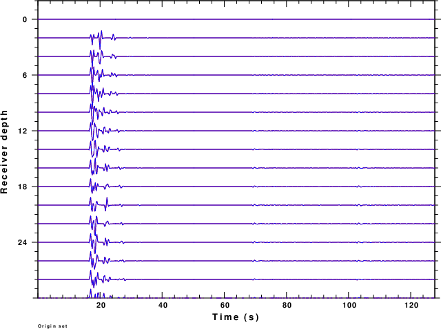
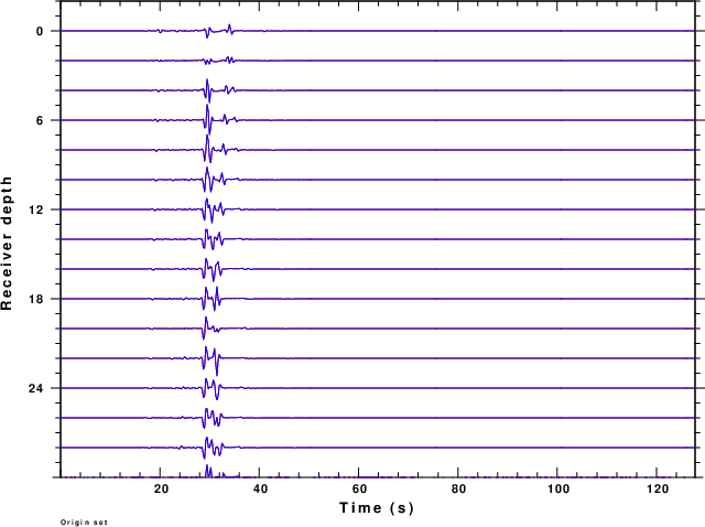
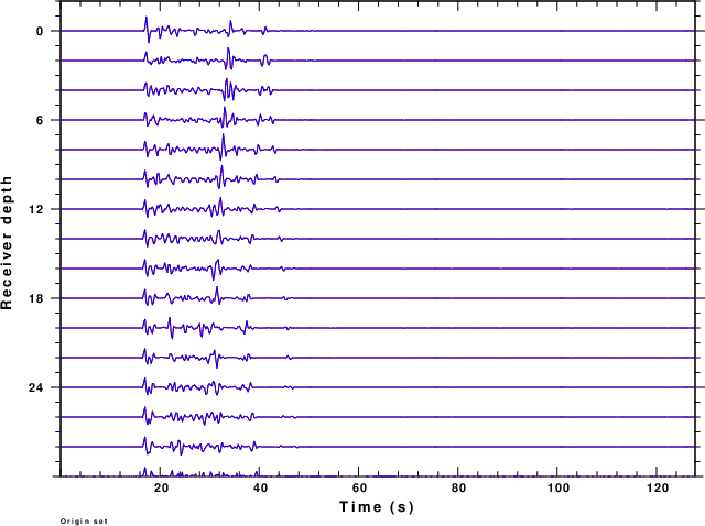
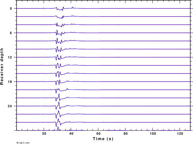
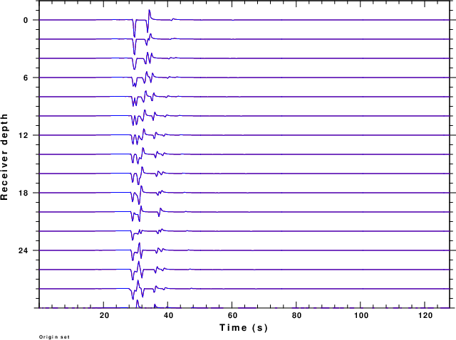
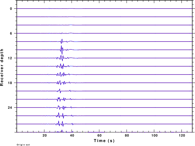
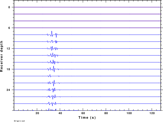
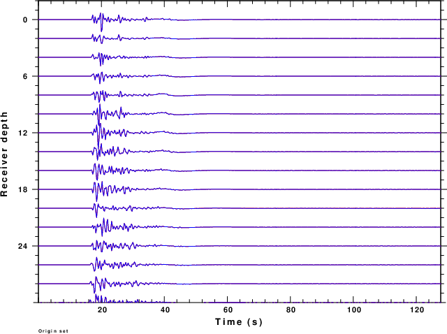
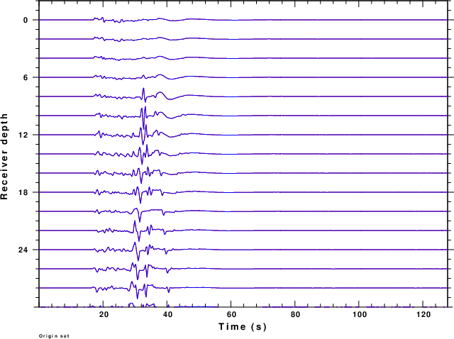
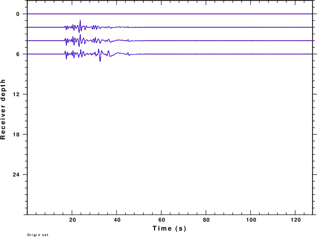
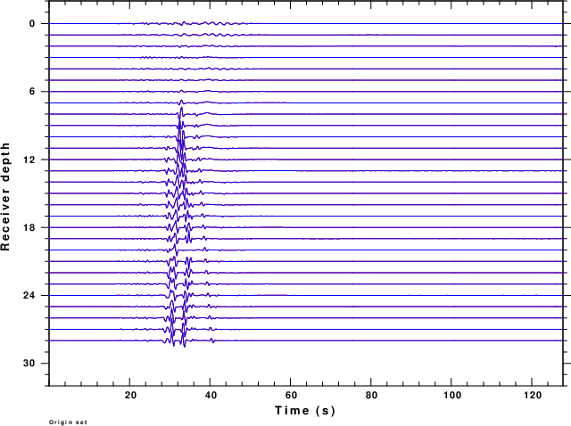
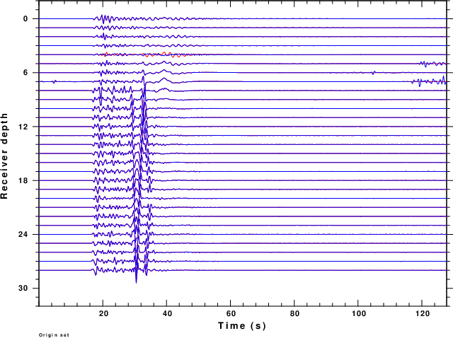
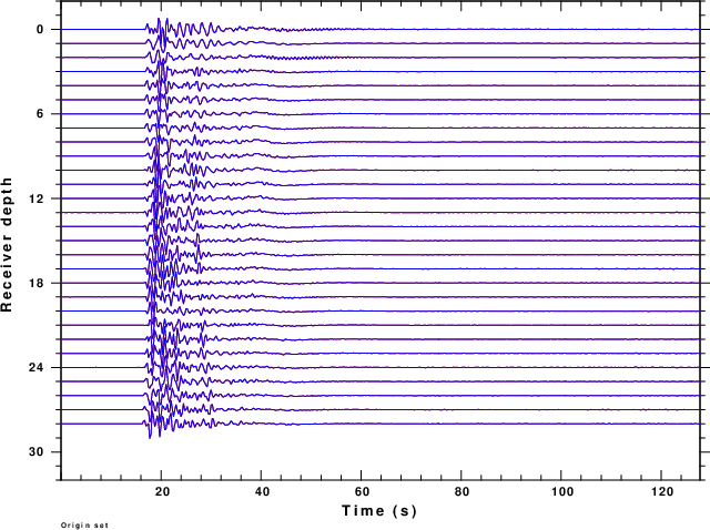
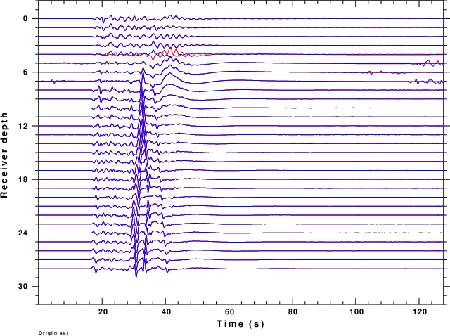
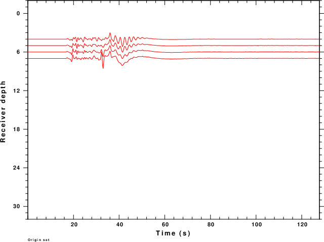
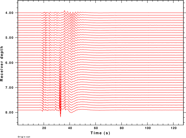
  H(KM) VP(KM/S) VS(KM/S) RHO(GM/CC)   QP   QS  ETAP  ETAS  FREFP  FREFS
  4.0000  6.0000  3.5000  2.7000 0 0 0 0 1 1
  4.0000  6.0000  3.5000  2.7000 0 0 0 0 1 1
  7.0000  6.0000  3.5000  2.7000 0 0 0 0 1 1
 26.0000  6.0000  3.5000  2.7000 0 0 0 0 1 1
   .0000  8.0000  4.7000  3.3000 0 0 0 0 1 1
For this model the ZDD, RDD, ZDS, RDS, TDS, ZSS, RSS, TSS, ZEX, REX, ZVF, RVF, ZHT, RHF and THF Green's functions are created. The source is at a depth of 20 km and the receiver depths vary from the surface to 30 km. The rspec96 and hspec96 Green's functions are plotted in red and blue, respectively. The plots are a true amplitude plot, meaning that the relative amplitudes between rceiver depths is preserved. Click on the links to see the comparison.
The display shows only subtle differences between the results of the two methods.
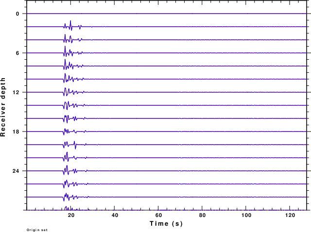
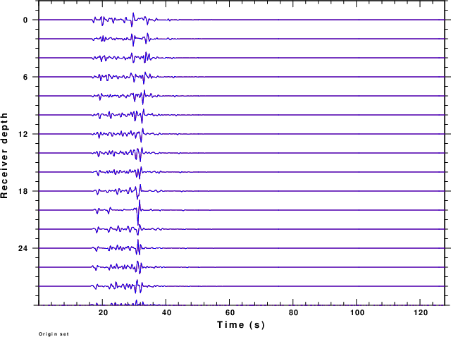
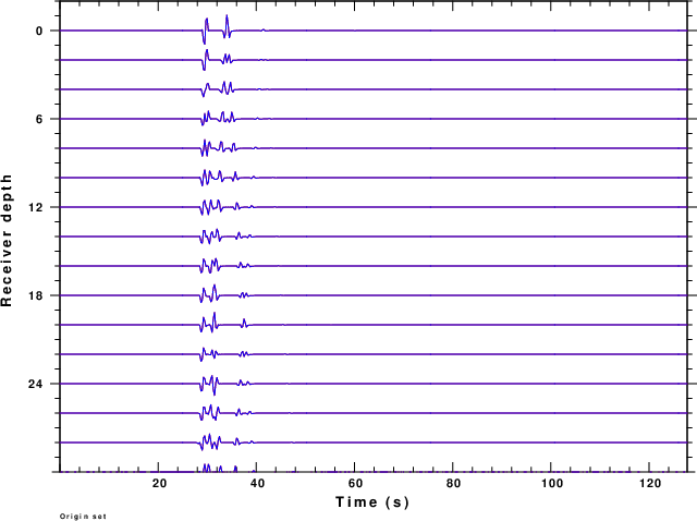
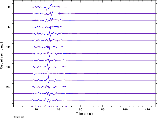
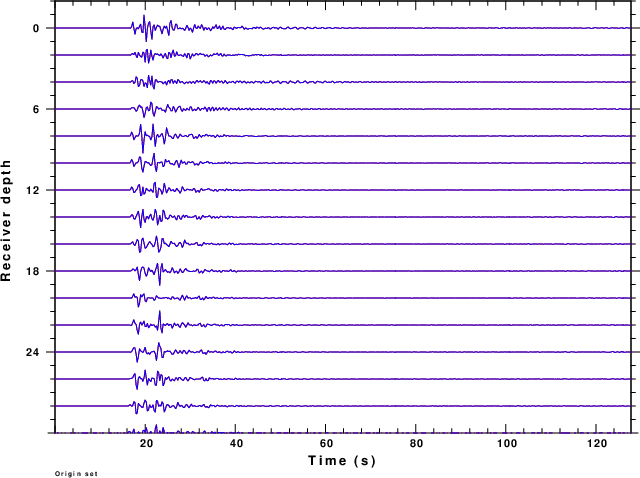
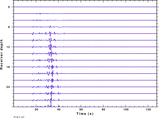
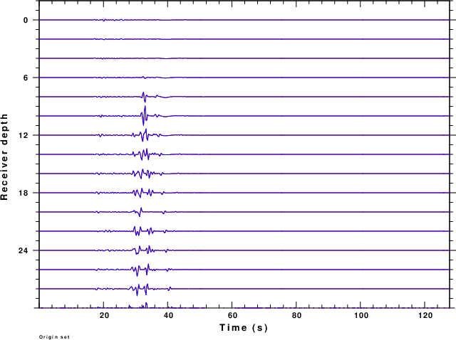
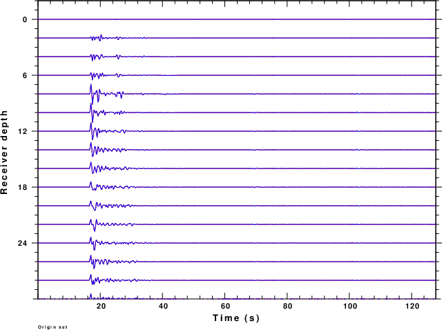
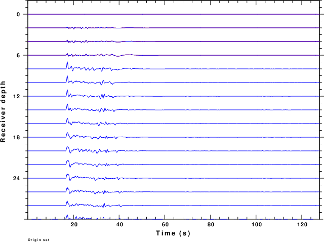
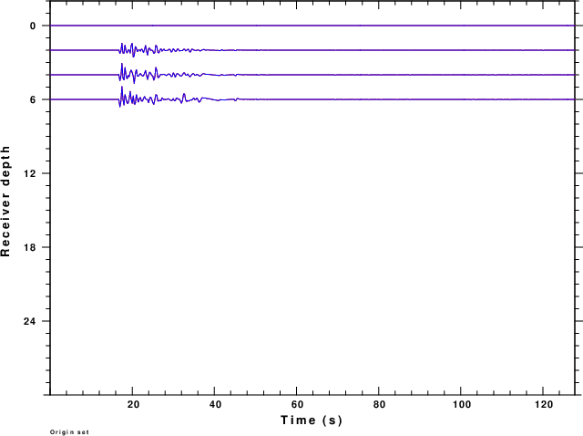
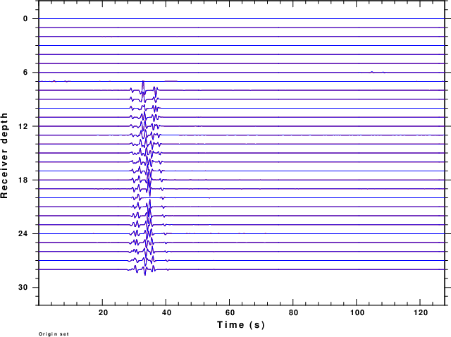
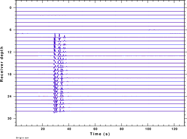
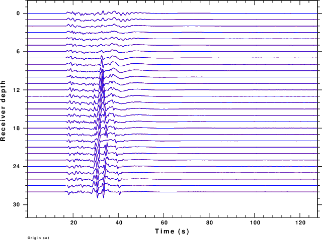
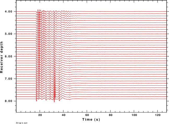
  H(KM) VP(KM/S) VS(KM/S) RHO(GM/CC)   QP   QS  ETAP  ETAS  FREFP  FREFS
  4.0000  6.0000  3.5000  2.7000 0 0 0 0 1 1
  4.0000  6.0000  3.5000  2.7000 0 0 0 0 1 1
  7.0000  6.0000  0.0000  2.7000 0 0 0 0 1 1
 26.0000  6.0000  0.0000  2.7000 0 0 0 0 1 1
   .0000  8.0000  0.0000  3.3000 0 0 0 0 1 1
For this model only the ZEX, REX and PEX Green's functions are created since the source is in the fluid. The PEX Green's function is created only for the receiver in the fluid. The source is at a depth of 20 km and the receiver depths vary from the surface to 30 km. The rspec96 and hspec96 Green's functions are plotted in red and blue, respectively. The plots are a true amplitude plot, meaning that the relative amplitudes between rceiver depths is preserved. Click on the links to see the comparison.
The display shows only subtle differences between the results of the two methods.
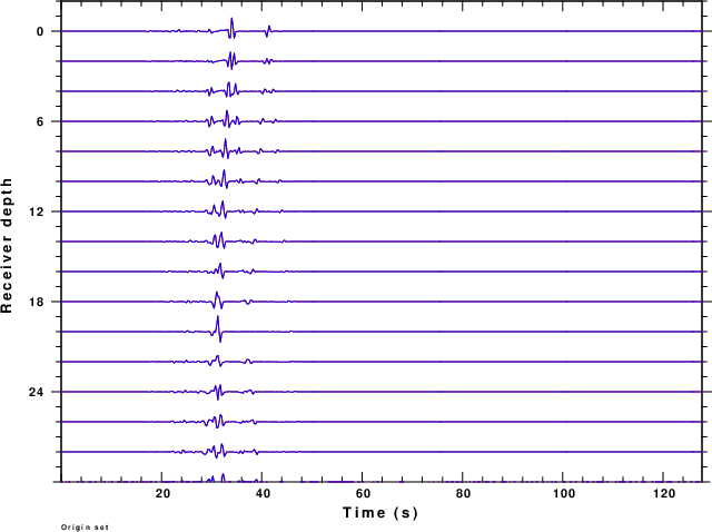
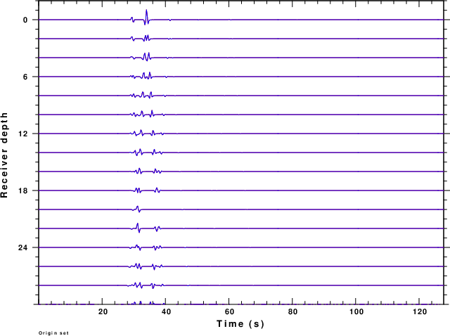
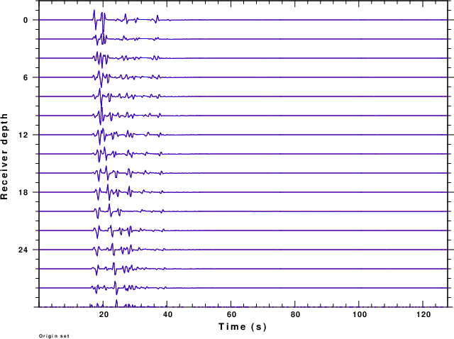
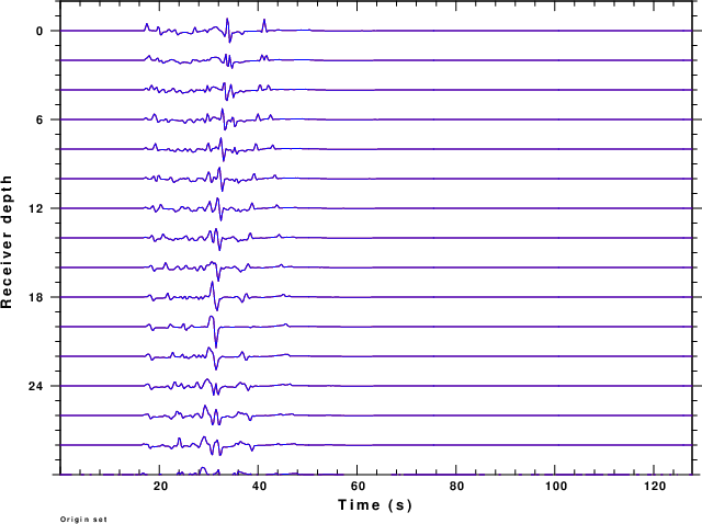
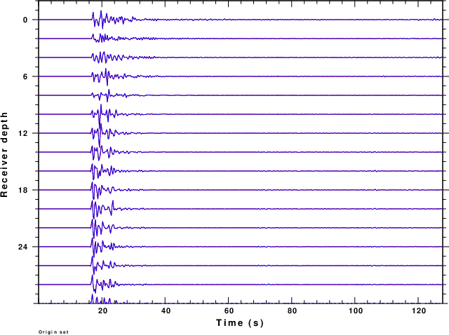
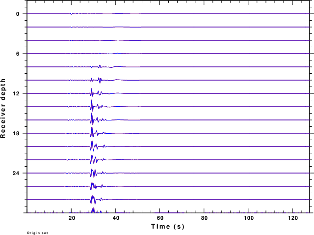
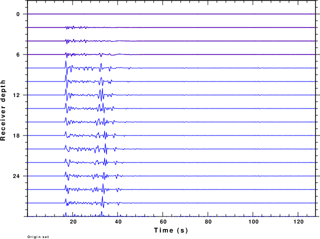
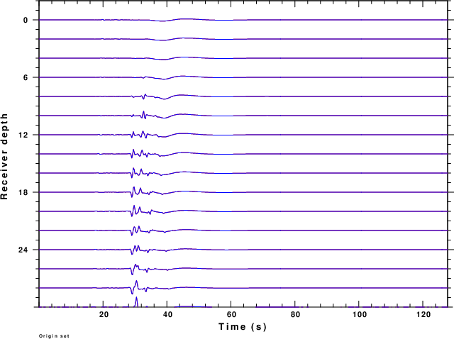
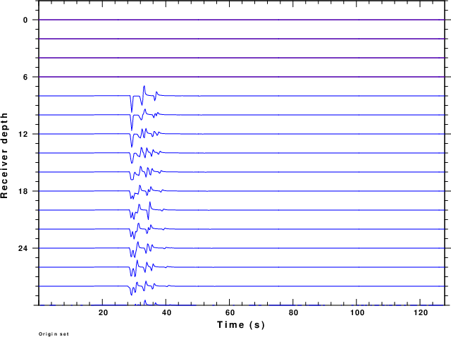
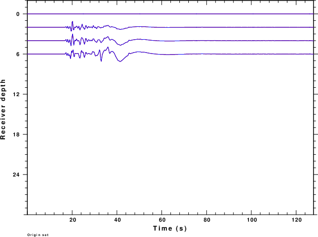
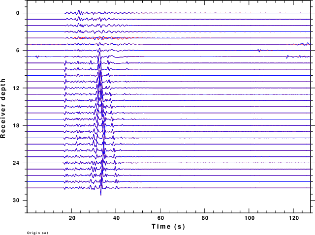
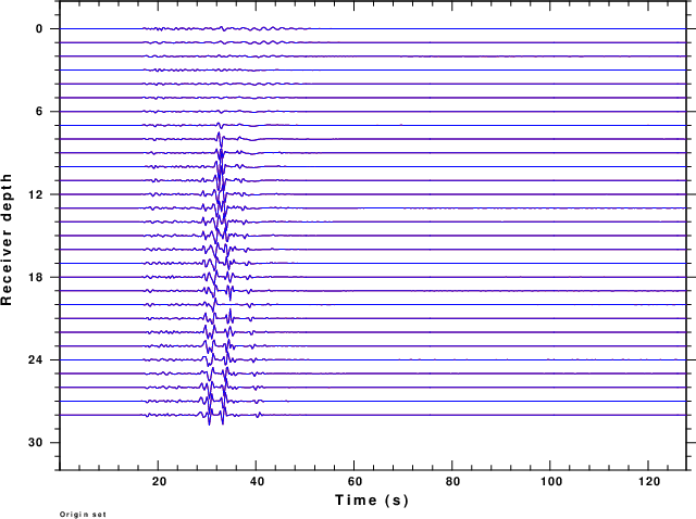
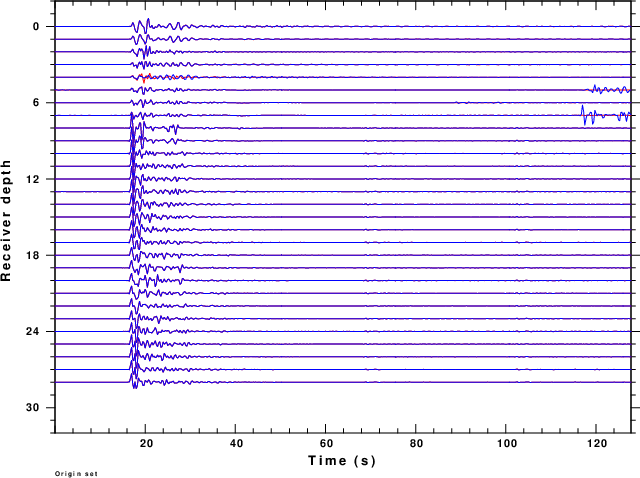
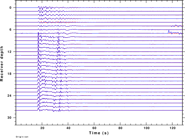
  H(KM) VP(KM/S) VS(KM/S) RHO(GM/CC)   QP   QS  ETAP  ETAS  FREFP  FREFS
  4.0000  6.0000  0.0000  2.7000 0 0 0 0 1 1
  4.0000  6.0000  0.0000  2.7000 0 0 0 0 1 1
  7.0000  6.0000  3.5000  2.7000 0 0 0 0 1 1
 26.0000  6.0000  3.5000  2.7000 0 0 0 0 1 1
   .0000  8.0000  4.7000  3.3000 0 0 0 0 1 1
For this model the ZDD, RDD, ZDS, RDS, TDS, ZSS, RSS, TSS, ZEX, REX, ZVF, RVF, ZHT, RHF, THF, PDD, PDS, PSS, PEX, PVF and PHF Green's functions are created. The source is at a depth of 20 km and the receiver depths vary from the surface to 30 km. The rspec96 and hspec96 Green's functions are plotted in red and blue, respectively. The plots are a true amplitude plot, meaning that the relative amplitudes between rceiver depths is preserved. Click on the links to see the comparison.
The display shows only subtle differences between the results of the two methods. Note that the P?? are not computed at a receiver depth of 8 km since the code computes the response on the solid side of tat boundary, e.g., at 8+ km.
| S.mod |
Sa.mod |
Sb.mod |
MODEL.01 |
MODEL.01 |
MODEL.01 |
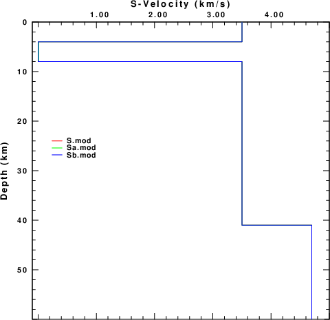
The next figure plots the Shear velocities of these models. Since
the S-velocities in the second layer are very small, their
differences are not seen in the figure.
|
To compare results of the different codes, the computations make
using a single ray parameter with hspec96p or rspec96p
are the fastest, but for waveform modeling the complete synthetics
computed using hspec96 or rspec96 must be
computed. There is not too much difference in the execution times
of these codes.
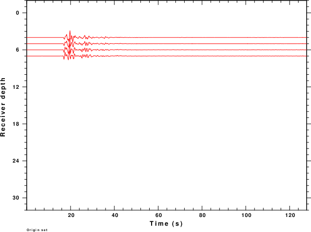
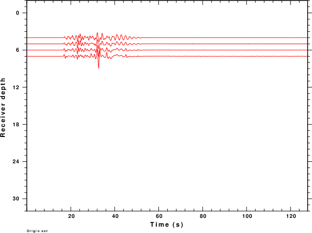
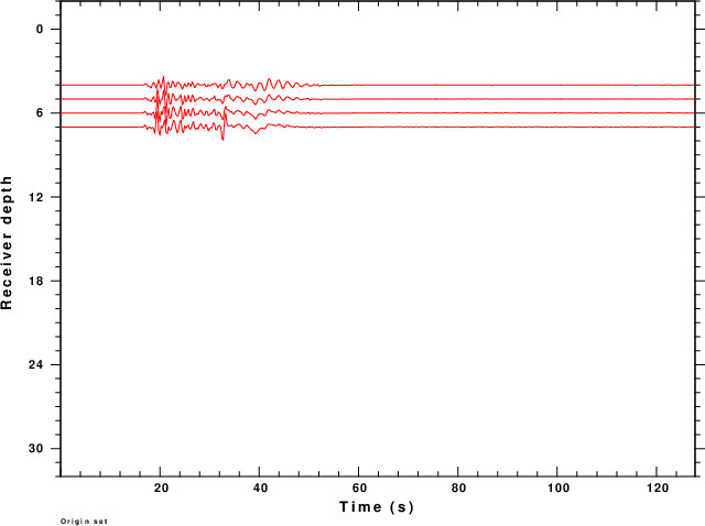
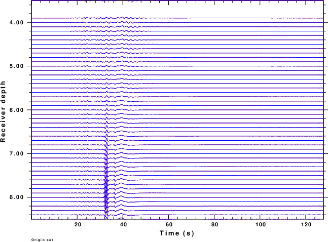
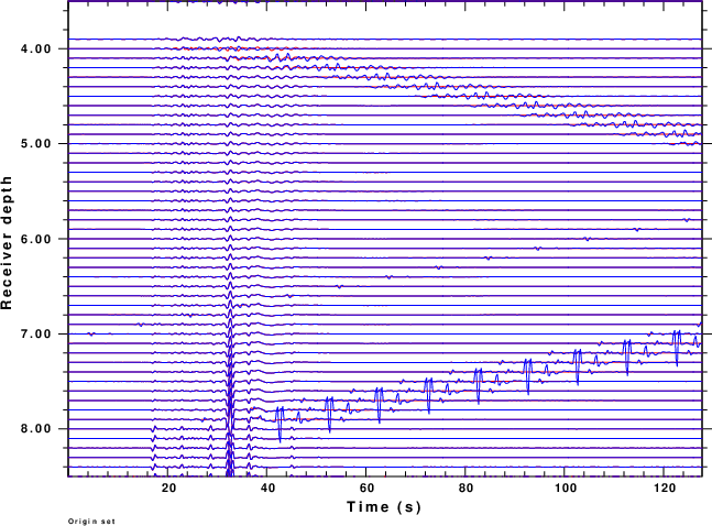
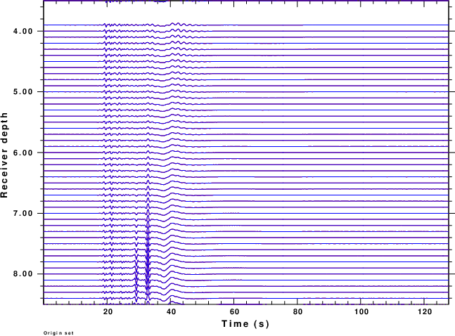
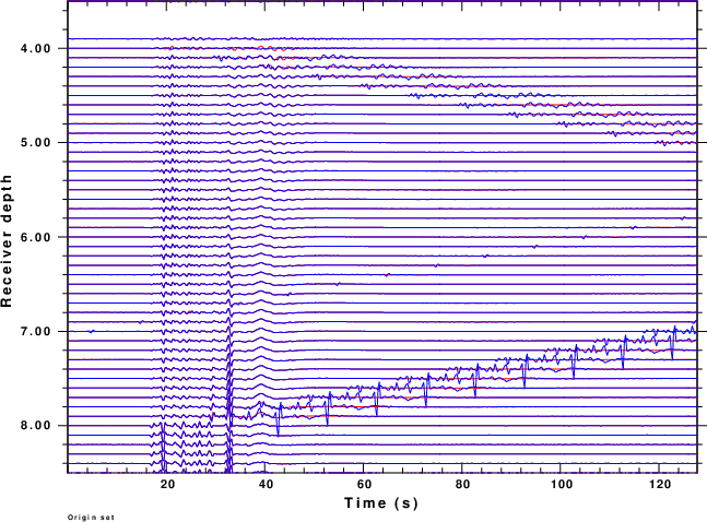
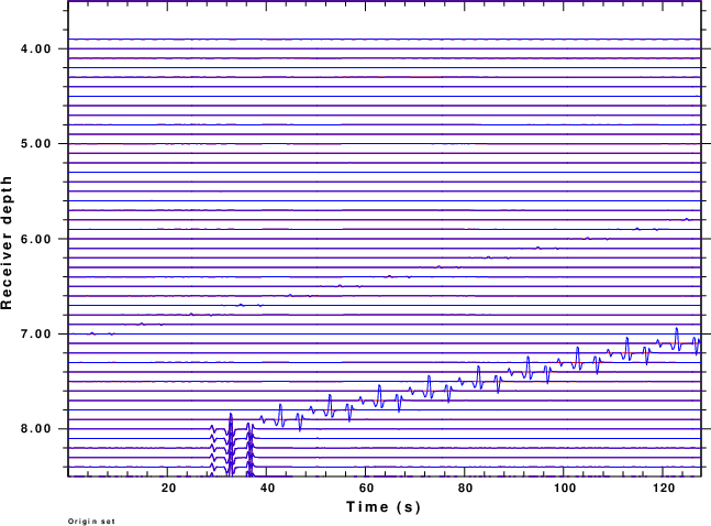
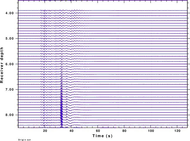
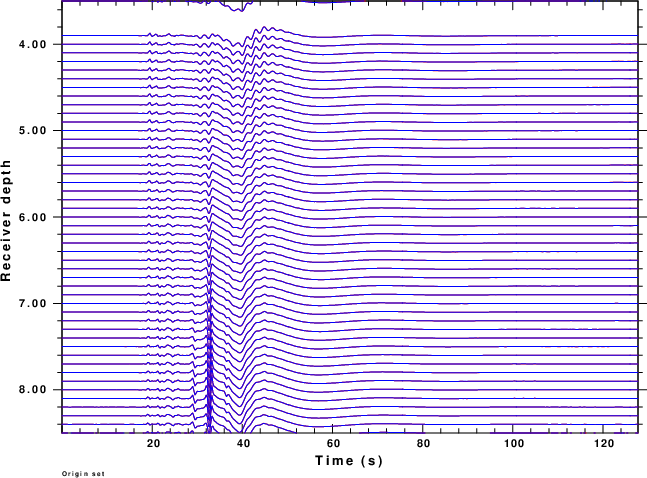
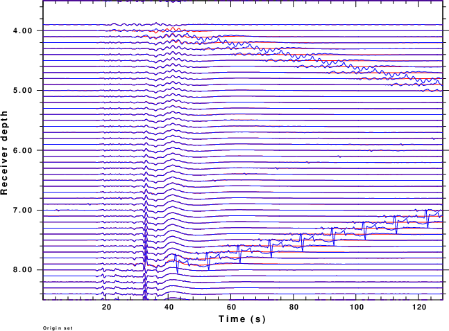
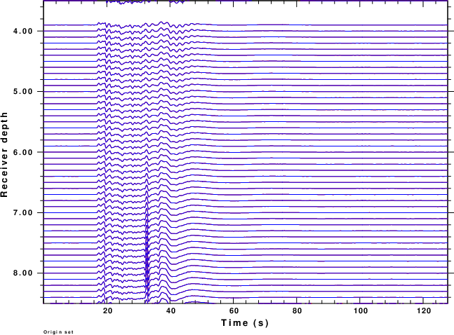
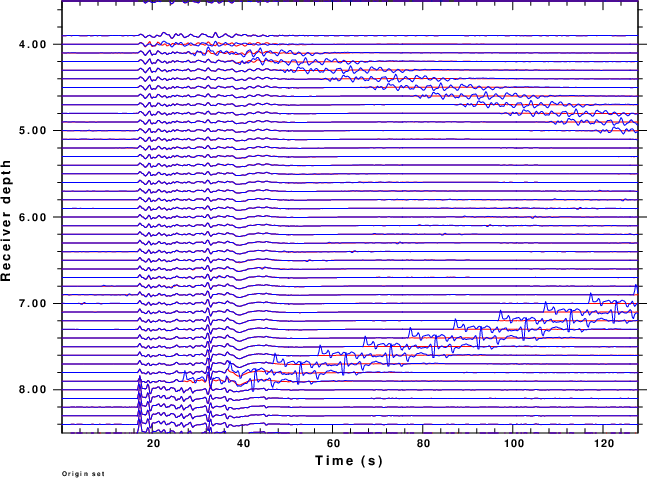
For this comparison the S.mod is used with rspec96 and Sa.mod with hspec96.
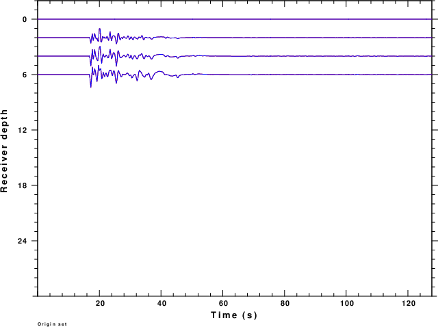
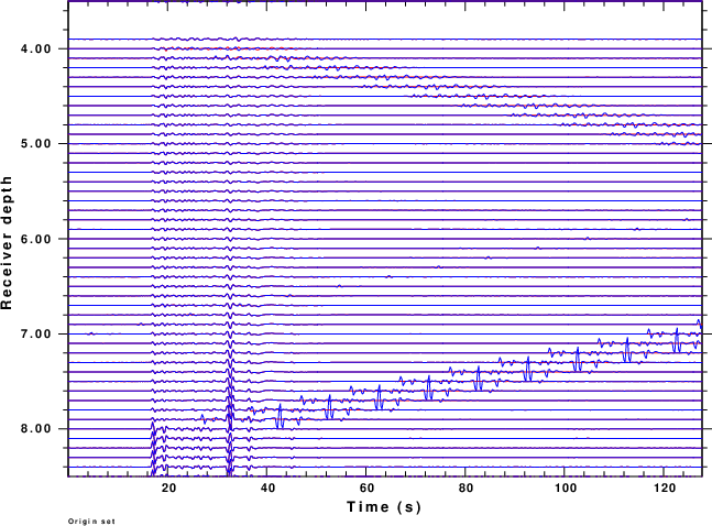
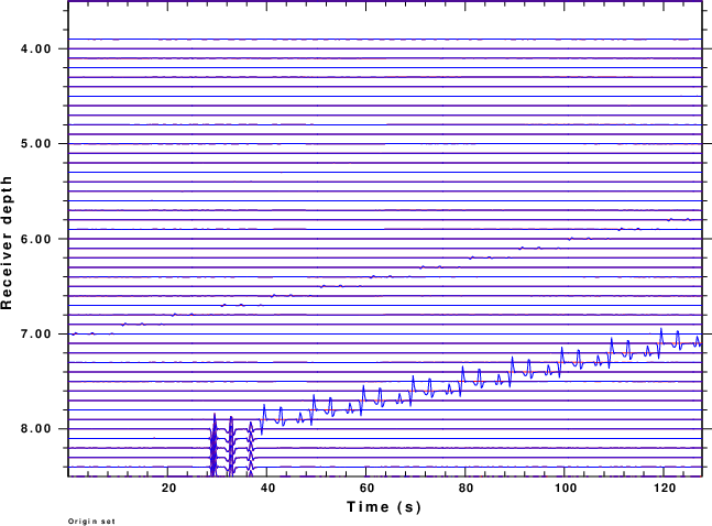
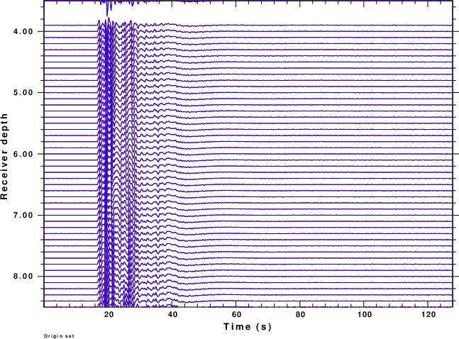
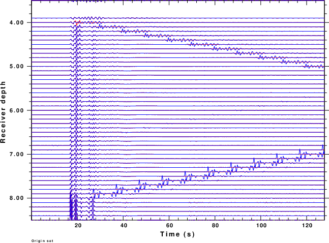
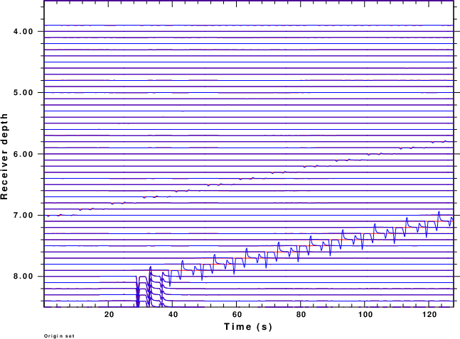
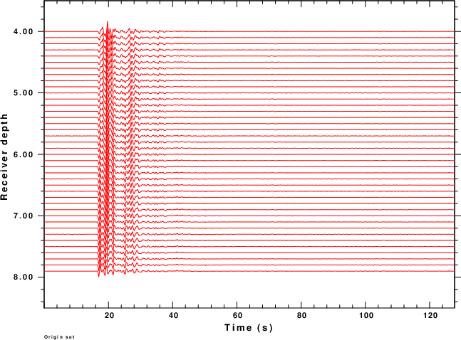
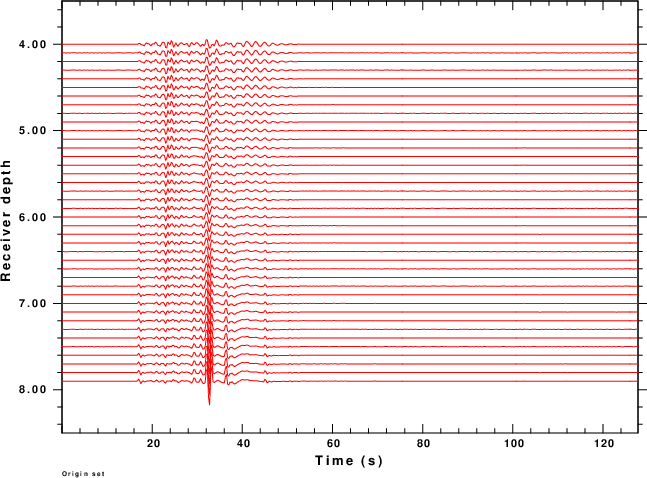
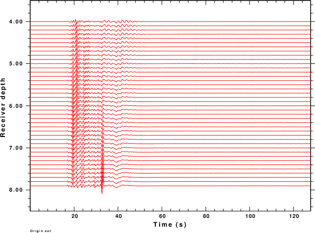
In the trace comparisons the only real differences are in the R?? components. For example look at the REX Grens/ function at 5 and 7 km at late times. These would be a problem is a shorter time window were used because of the periodicity of the FFT used. Note that these later arrivals are about 100 sec after the first P arrival.
Click on the links to see the comparison. Note the P?? are componented only for the rspec96 since the Sa.mod is a solid model even though the S velocity is very small.
These plot focus on the arrivals in the water layer. Remembering that the color blue is used for the hspec96 synthetics. A set of arrivals is genereated at the sharp velocity boundary at 4 and 8 km. The moveout indicates that these are the S-wave propagating at 0.01 km/sec. In genereal the initial part of the traces agree very well. It is only at location near the boundary that these arrivals interfer with the expected motion.
One cannot make the S velocity too small to simulate a fluid when using hspec96 if the computations are done in single precision.
The other conclusion is that the Z?? displacements in the fluid comapre well. Although the hspec96 will not give the P?? in the fluid, the displacements in the overlying solid are correctly computed. This one could use hspec96 for the ice/water/solid problem.
Click on the links to see the comparison.
One subtle difference in the implementation occurs when the
source or receiver depth is at the solid/liquid boundary, e.g., at
a depth of 4.0 or 8.0 km in the S.mod above.
Actually in the code, the decision is whether the
observation point is at the bottom of the layer above or at the
top of the layer below. One could follow the code, but one could
also experiment by computing synthetics at just above and
below the boundary and then comparing those to the synthetics
computed at the boundary, This distinction is pertinent
since the vertical displacement and stress are continuous across a
fluid/solid boundary, but the radial displacement is not.
I mention this because of the use of OBS platforms. Thus to make
synthetics for the particle velocities, I would perform the
computations at a depth of about 1 meter or so below the
ocean/solid boundary. To get the pressure field, I would run the
codes for a receiver in the fluid at a height of about 1 meter
above the boundary.