Computer Programs in Seismology

Strain Synthetics - Tests - II

1. Introduction

This tutorial introduces the programs sshspec96 and sshspec96strain which make use of a property of real causal functions that states that

where U(t) is the unit step function. This relation arises from the decomposition of a real function into even and odd parts, e.g., h(t) = h_e(t) + h_o(t) and for real h(t), its Fourier transform is H(ω) = R_e(ω) + i I_o(ω). If there is no discontinuity at t=0, then h_o(t) = sgn(t) h_e(t) and h_e(t) = sgn(t) h_o(t), which says that R_e(ω) and I_o(ω) are Hilbert transforms of each other in the frequency domain.

When solving wave equation problems in cylindrical coordinates, one has

The advantage of this expression is that it is not necessary to integrate to infinity for non-attenuative media since Im H(k,ω) = 0 for k > k_max, where k_max=ω/V_min and V_min is the lowest P- or S-wave velocity. This is useful when the source and receiver are at the same depth, and the exponential decay in the H(k,ω). cannot be relied upon to truncate the integral.

This approach follows the work of Sánchez-Sezma et al (2011) in their study of H/V ratios from ambient noise. The reference is

Sánchez-Sesma, F. J., Rodríguez, M., Iturrarán-Viveros, U., Luzón, F., Campillo, M., Margerin, L., García-Jerez, A., Suarez, M., Santoyo, M. A., and Rodríguez-Castellanos, A. (2011). A theory for microtremor H/V spectral ratio: application for a layered medium:. Geophys. J. Int., 186:221-225.

In order to implement this technique to compare to N-point synthetics created by hspec96 and hspec96strain, a 2N point time series must be used with sshspec96 and sshspec96strain, and then the first half of the time series saved. This truncation step is required since negative values map into the second half of the trace.

The reason for developing sshspec96 and sshspec96strain is to create synthetics efficiently for the special case that the source and receiver depths are identical.

Testing

The purpose of this tutorial is to compare sshspec96strain to hspec96strain focusing on the special case when the source and receiver depths are the same. The testing considers a set of epicentral distances for a fixed source depth and a set of source depths for fixed epicentral distance. As will be seen, the current code still has problems for some Green's functions at the vertical distance between the source and receiver is small.

An overview of the wavenumber integration and considerations in its implementation are given in the document Theory.pdf. The details about using the features of causality of real time functions, and hence the integration of Im H(k,ω) are given in lat02.pdf.

The test cases are given in STRAIN3.tgz. To run these yourself, do the following after downloading this archive:

gunzip -c STRAIN3.tgz | tar xf -
cd STRAIN3
DOALL

The results will be in directories such as ncVOLVInew/COMPAREZ.

2. Code test

The wavenumber integration code within hspec96, rspec96, tspec96 and hspec96strain often has numerical problems when the path of the direct arrival from the source to the receiver is nearly horizontal because the direct arrival is often has the largest amplitude and the small vertical offset means that the H(k,ω) does not decay rapidly as k → ∞. When the vertical offset is not zero, the decay occurs at high frequencies. The underlying difficulty is that wavenumber integration requires the evaluation of the integrals of the form ∫₀^∞ H ( k, ω ) J_n (k r ) dk, but this is approximated as ∫₀^k_max H ( k, ω ) J_n (k r ) dk assuming that the contribution from [k_max, ∞] is negligible. This truncation problem is worse at lower frequencies.

To test the current coding and to highlight problems, the Green's functions and partial derivatives with respect to the vertical and radial positions of the receiver are compared first with a fixed source depth of 10.0 km and different epicentral distances and then for a fixed radial distance of 10.0 km and different vertical distances between the source and the receiver. The use of hpulse96strain with the -TEST1 flag gives the Green's functions and the partial derivatives with respect to the receiver (r,z) coordinates. If these "look" good, then the strains, stresses and rotations computed will be OK. It is assumed that the computation of strain using the Green's functions and their derivatives with respect to 'r' and 'z' is correct.

Wholespace Test

The wholespace velocity model, named W.mod is created with this shell script:


cat > W.mod << EOF
MODEL.01
Simple wholespace model
ISOTROPIC
KGS
FLAT EARTH
1-D
CONSTANT VELOCITY
LINE08
LINE09
LINE10
LINE11
H(KM) VP(KM/S) VS(KM/S) RHO(GM/CC) QP QS ETAP ETAS FREFP FREFS
40.0  6.00       3.5     2.7        0  0  0    0     1     1
EOF

The processing scripts used are called with the source depth and epicentral distance as command line arguments.

#!/bin/sh H=$1 R=$2 cat > dfile << EOF ${R} 0.05 256 0 0 EOF hprep96 -M W.mod -d dfile -HS ${H} -HR 0 -TH -BH hspec96strain hpulse96strain -TEST1 -V -p -l 2 -FMT 2

#!/bin/sh H=$1 R=$2 cat > dfile << EOF ${R} 0.05 512 0 0 EOF hprep96 -M W.mod -d dfile -HS ${H} -HR 0 -TH -BH -XF 8 sshspec96strain hpulse96strain -TEST1 -V -p -l 2 -FMT 2 -HALF

#!/bin/sh H=$1 R=$2 cat > dfile << EOF ${R} 0.05 256 0 0 EOF hprep96 -M W.mod -d dfile -HS ${H} -HR 0 -TH -BH hwhole96strain hpulse96strain -TEST1 -V -p -l 2 -FMT 2

Note that the original time series for sshspec96strain is twice as long as that for hspec96strain and that the hprep96 has the flag -XF 8 so that the integration hopefully extends into the region where Im[ H(k,ω)] is effectively zero.

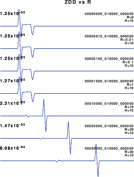
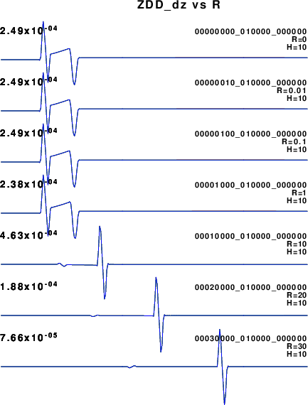
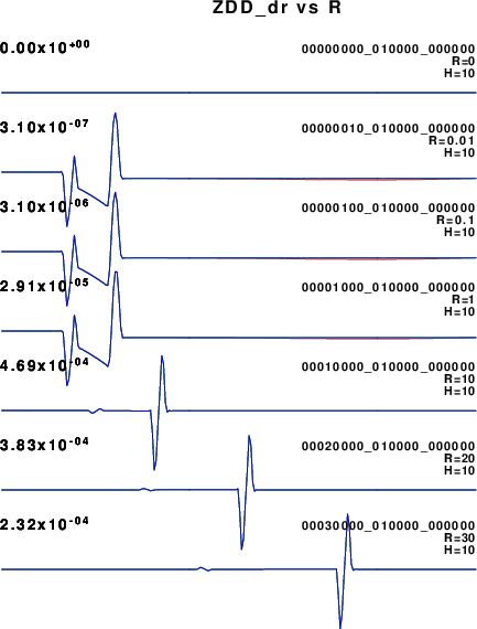
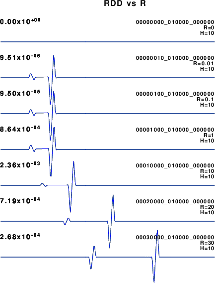
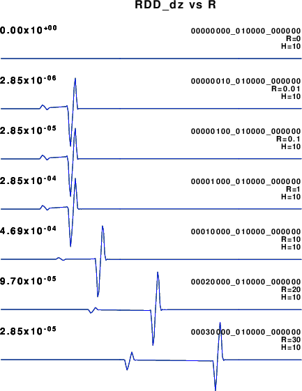
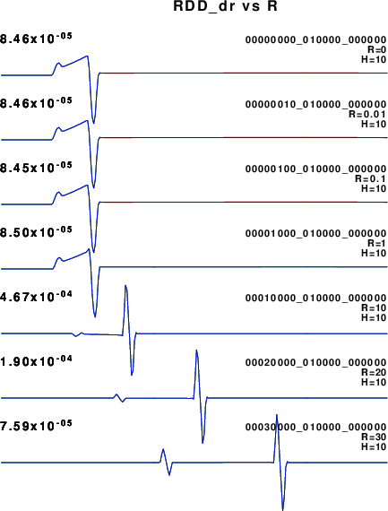
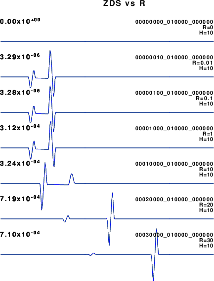
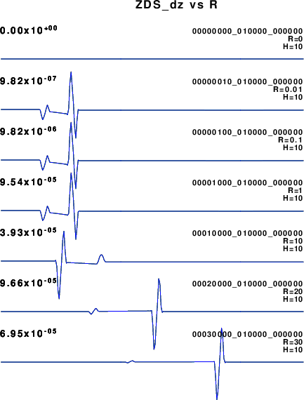
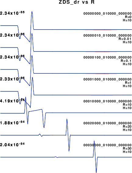
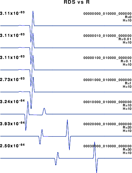
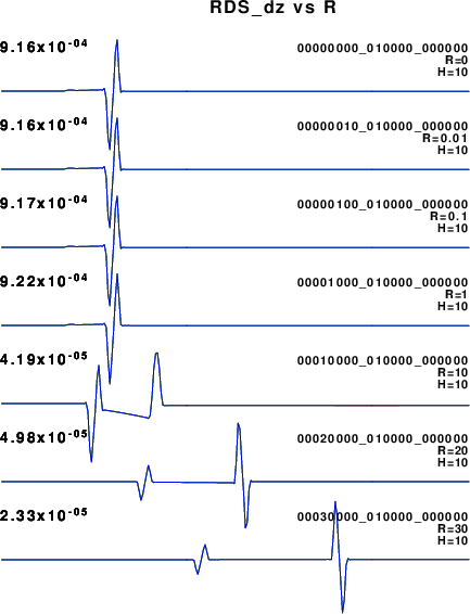
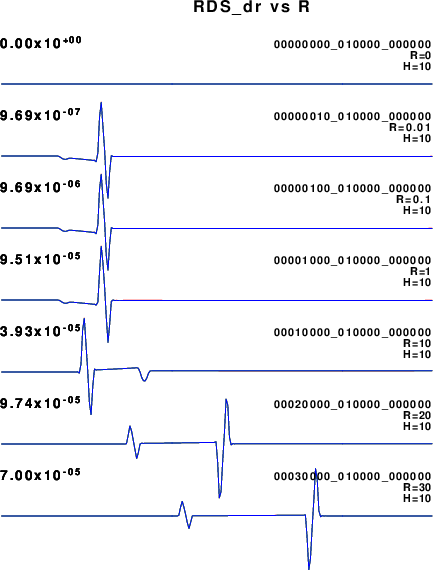
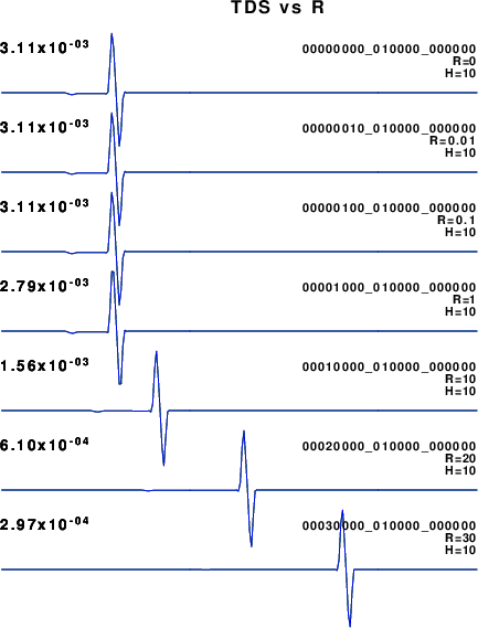
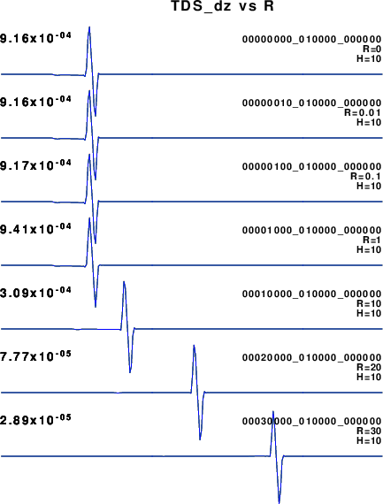
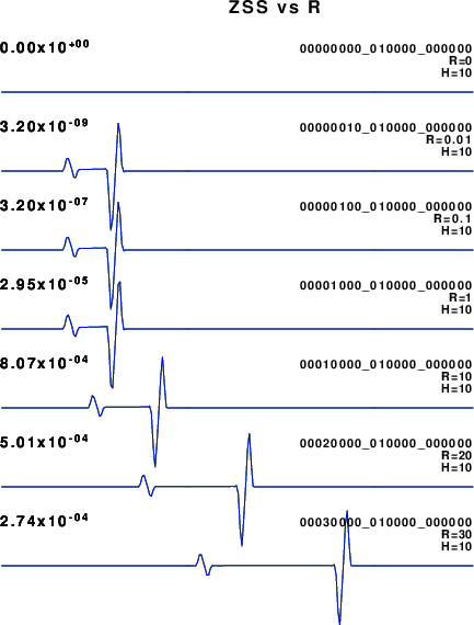
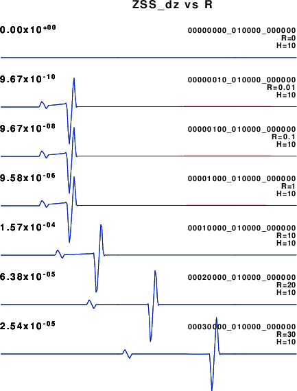
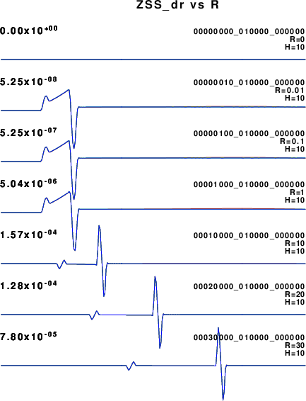
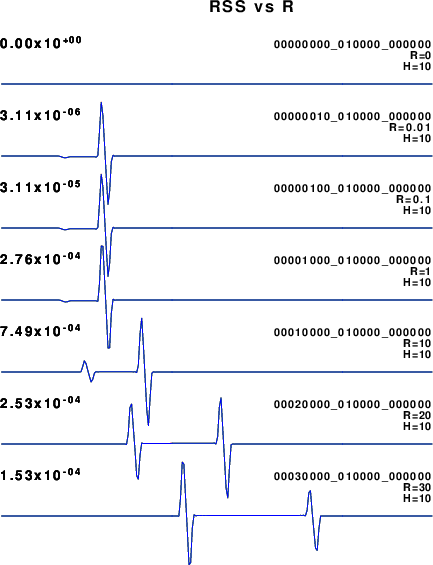
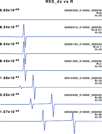
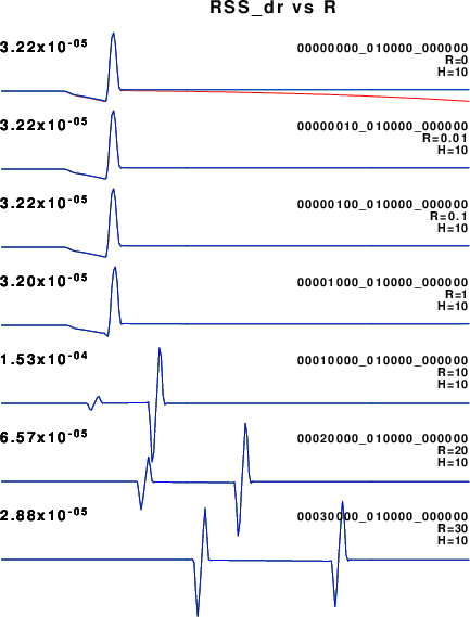
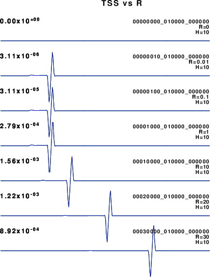
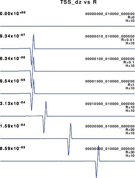
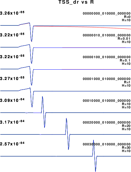
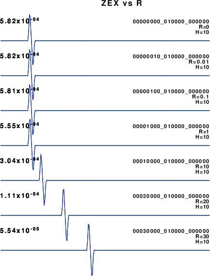
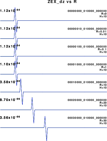
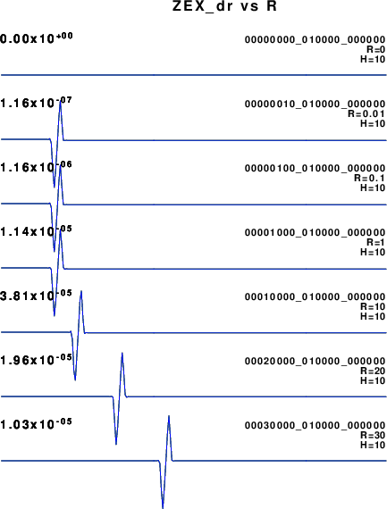
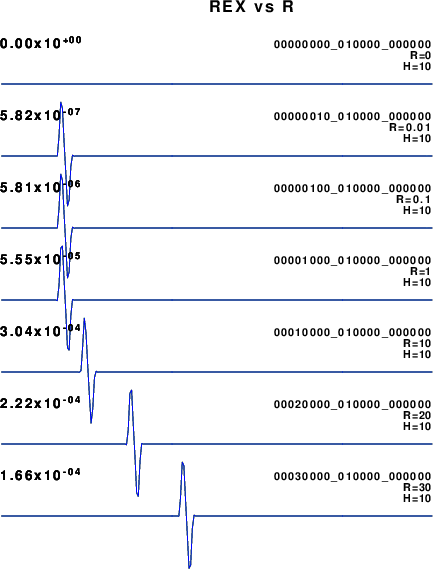
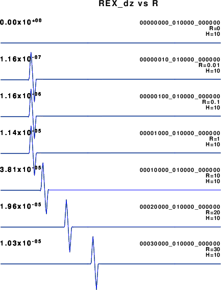
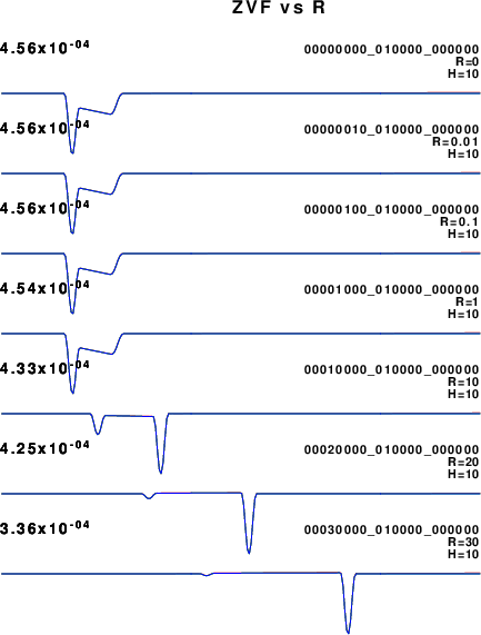
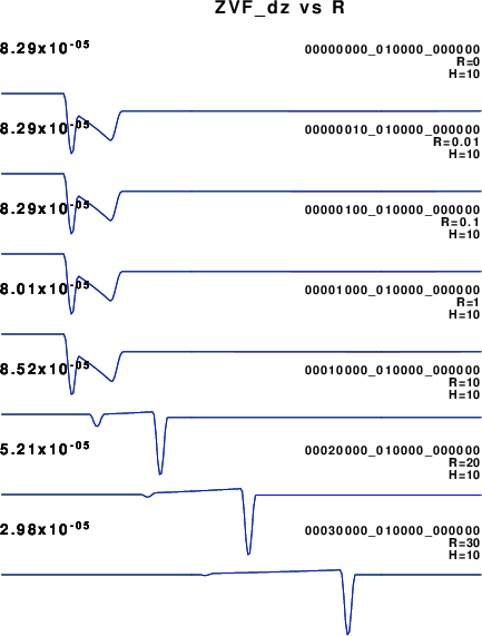
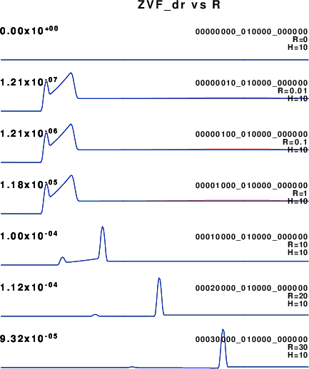
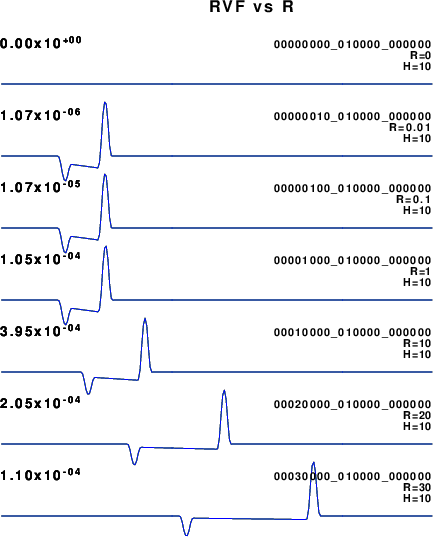
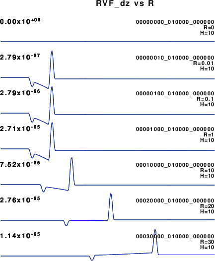
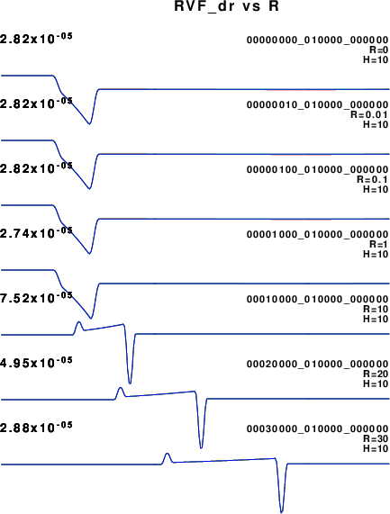
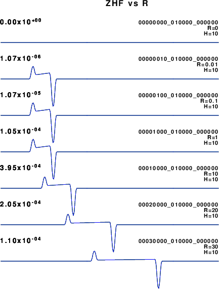
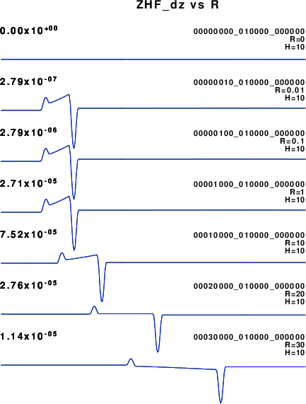
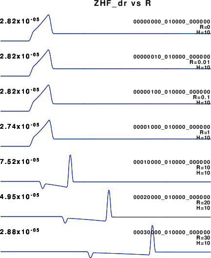
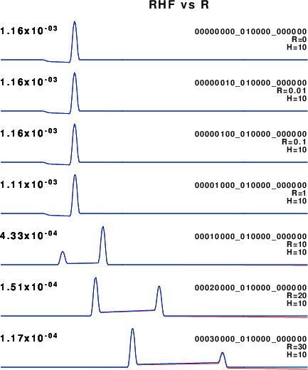
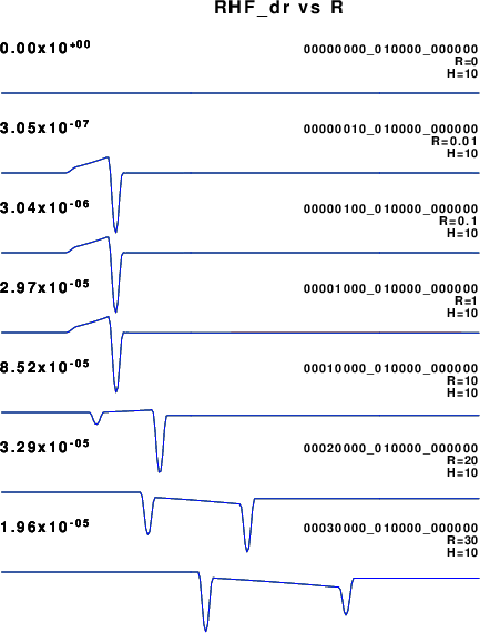
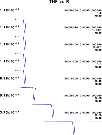
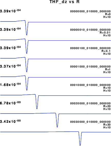
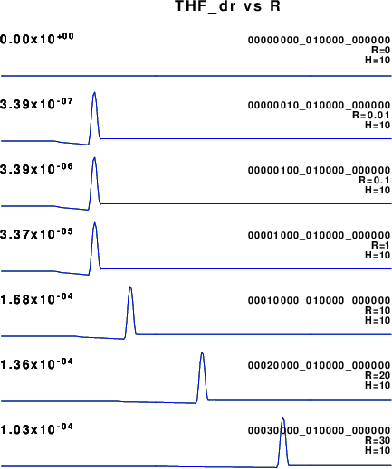
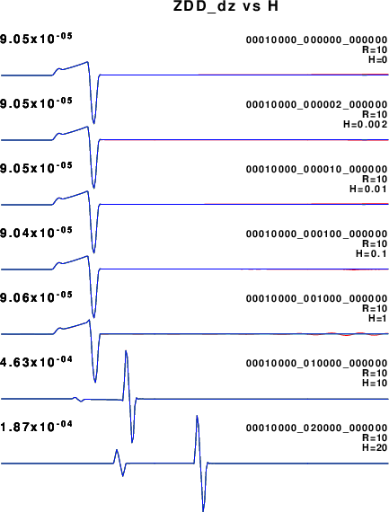
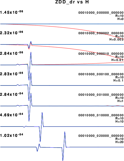
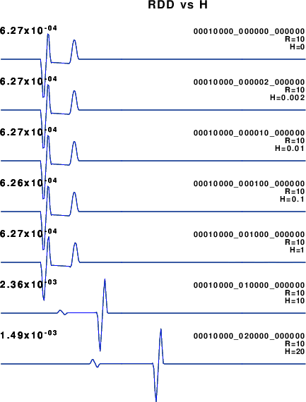
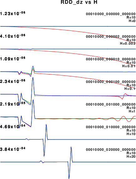
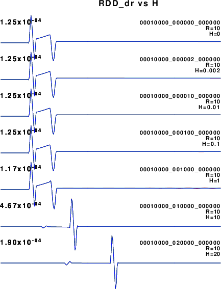
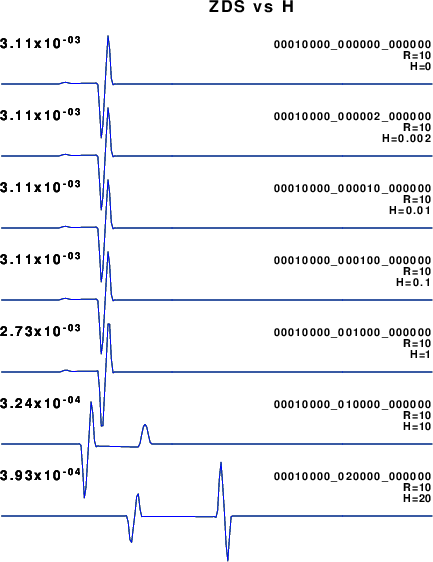
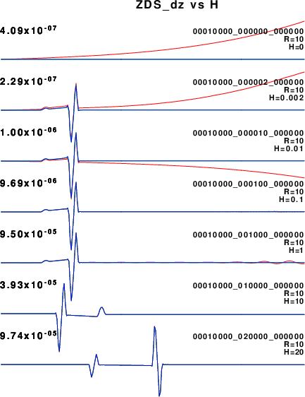
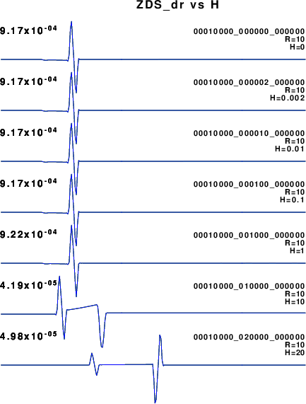
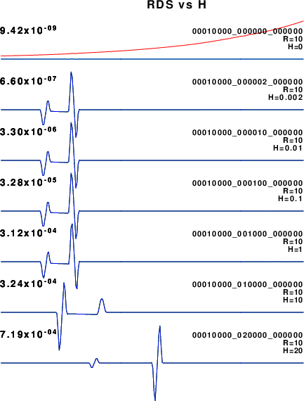
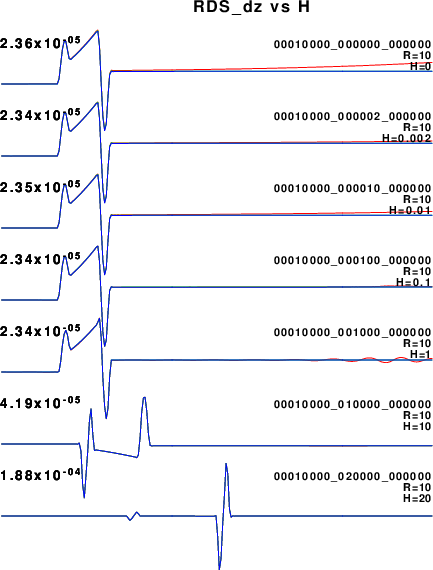
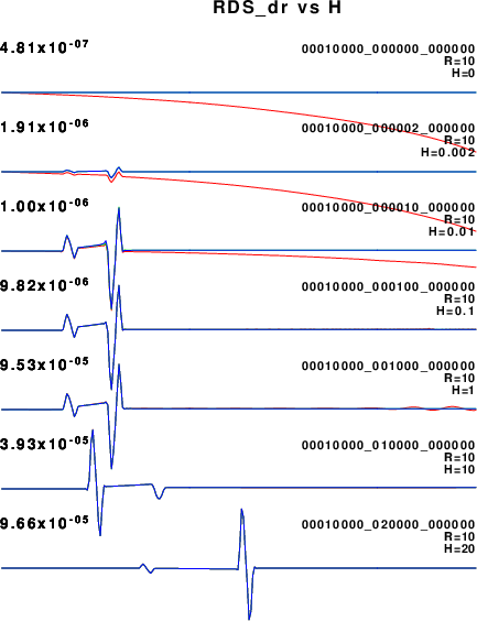
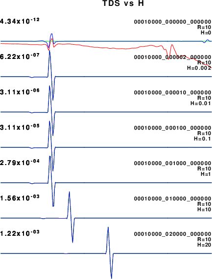
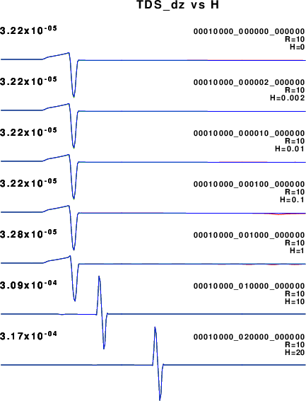
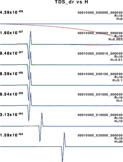
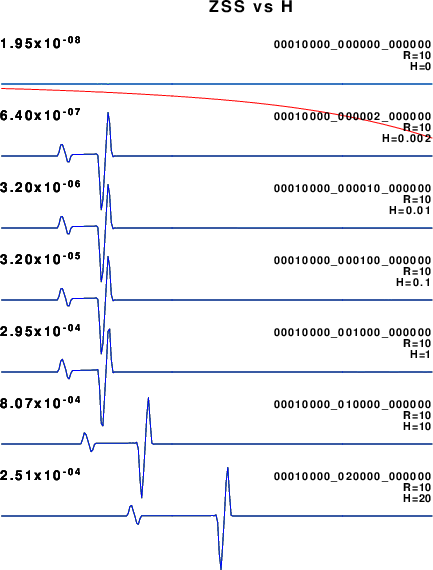
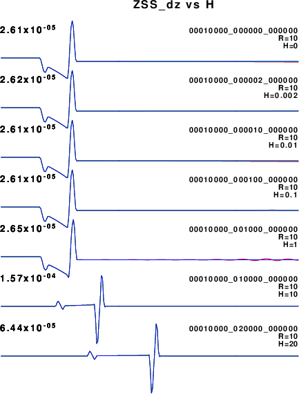
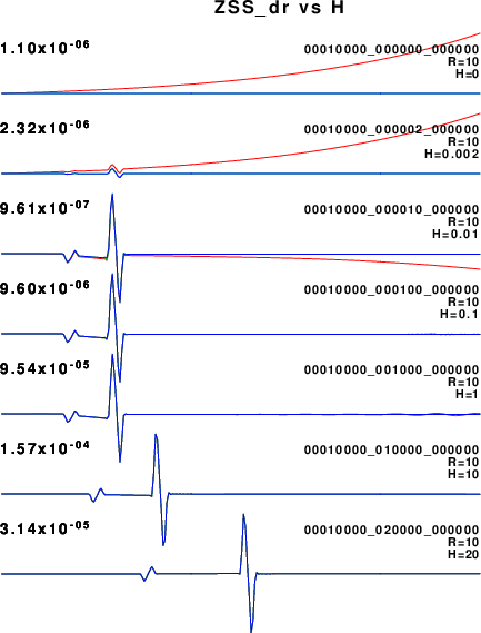
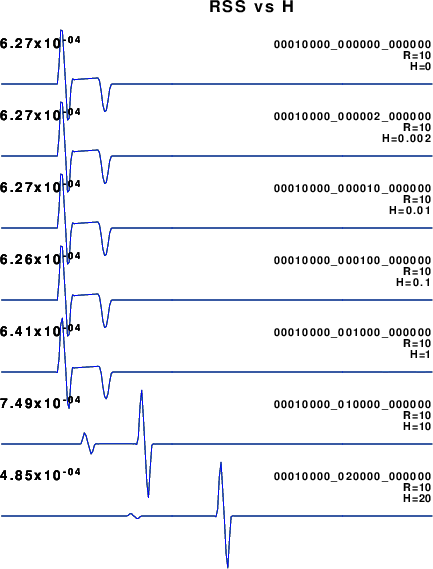
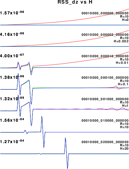
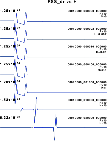
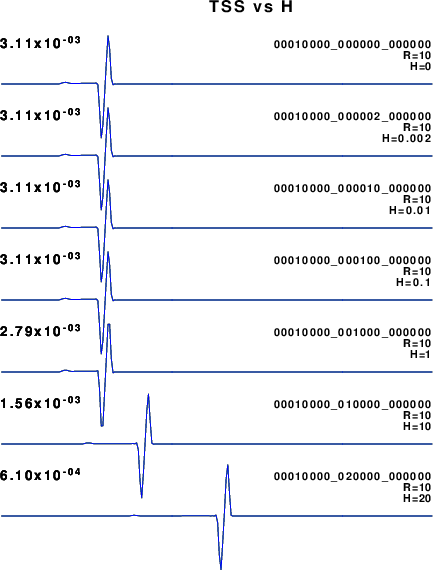
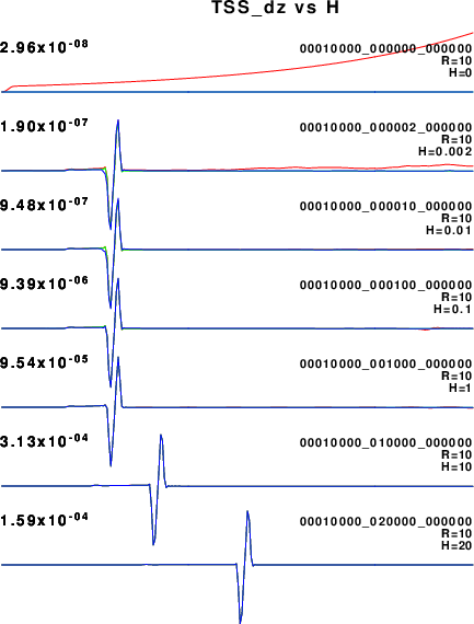
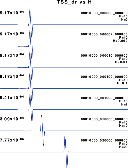
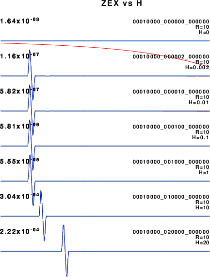
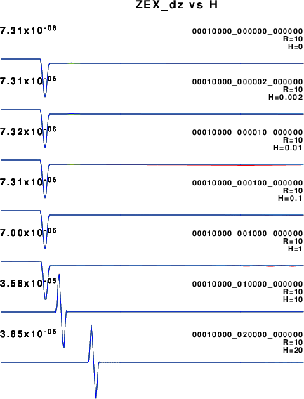
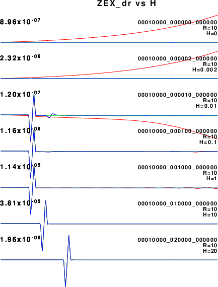
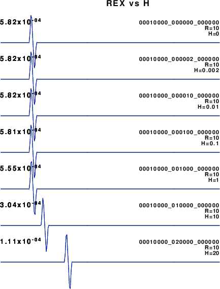
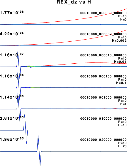
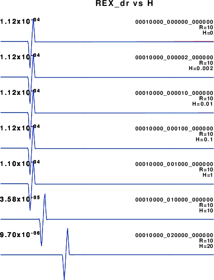
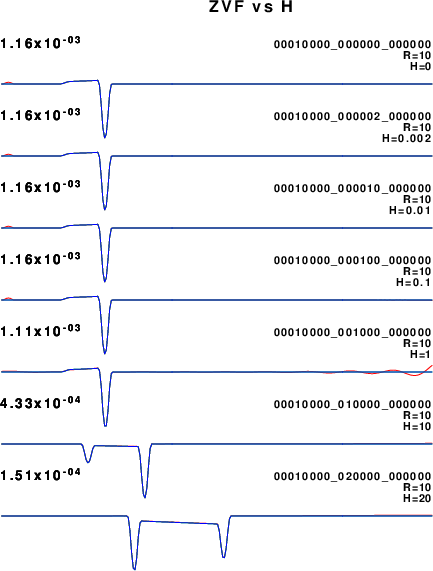
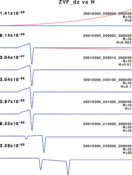
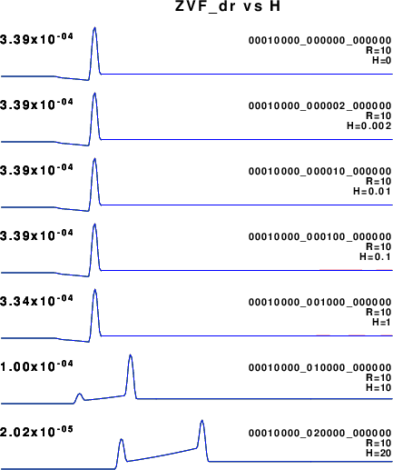
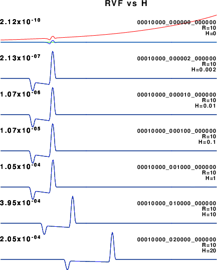
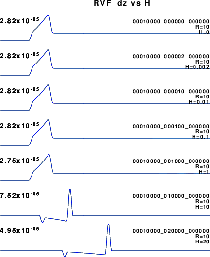
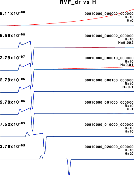
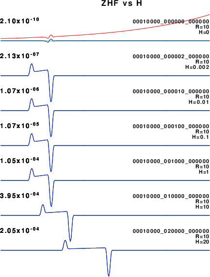
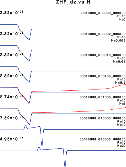
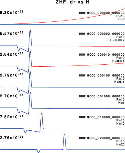
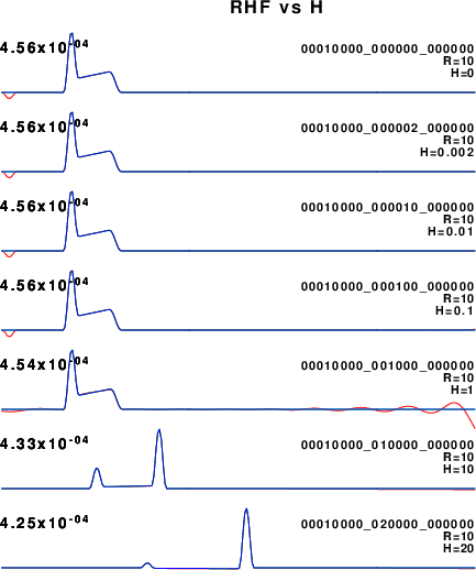
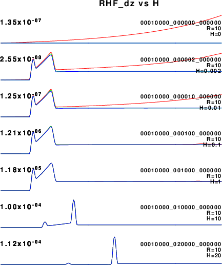
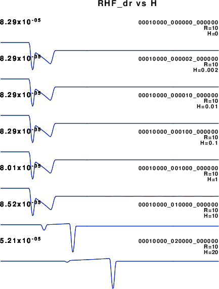
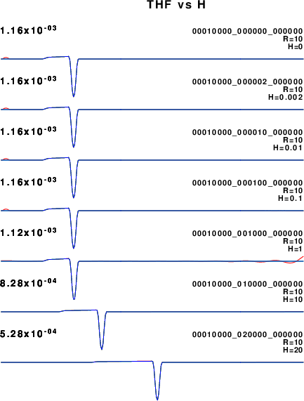
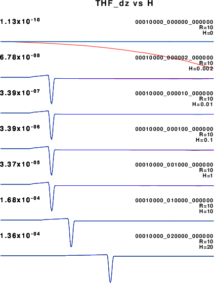
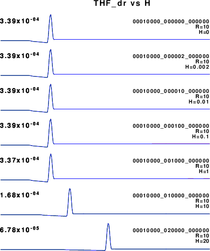
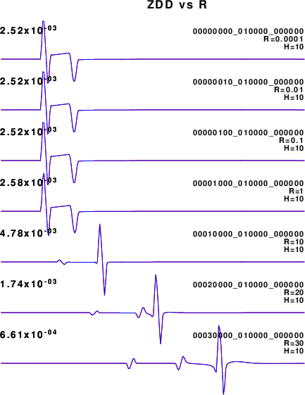
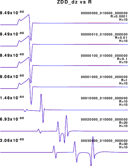
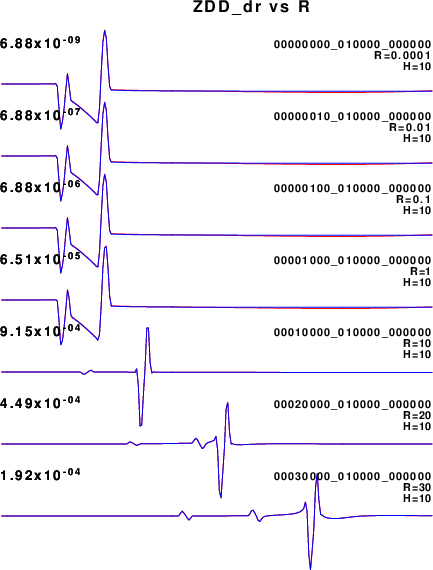
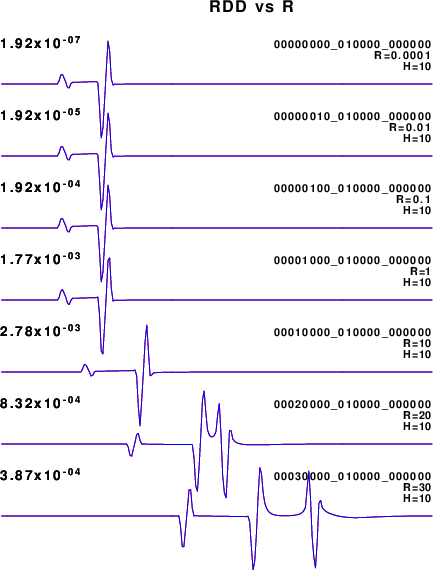
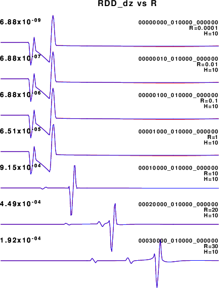
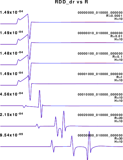
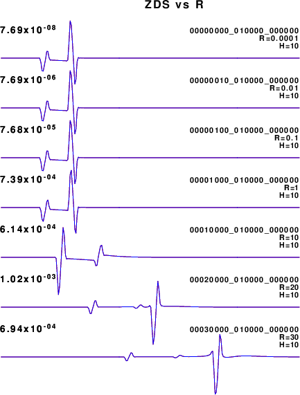
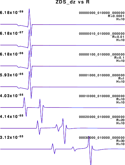
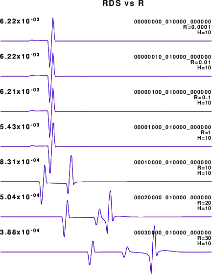
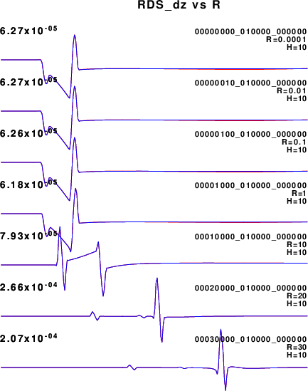
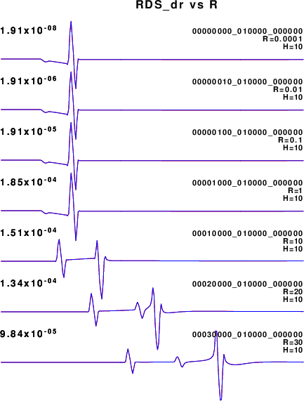
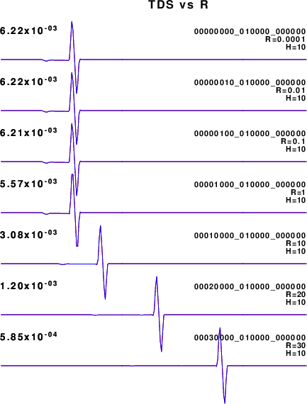
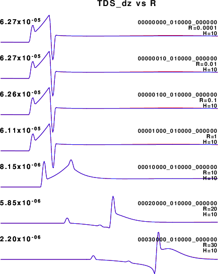
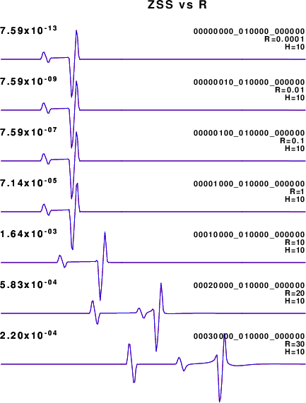
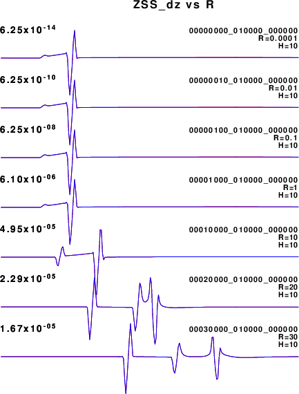
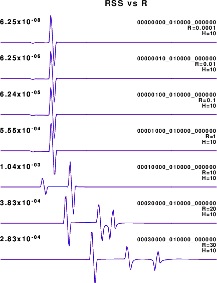
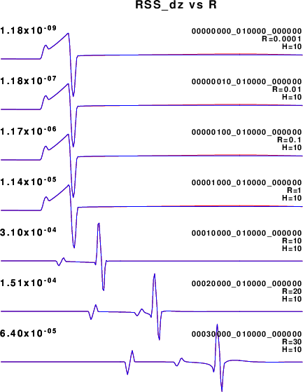
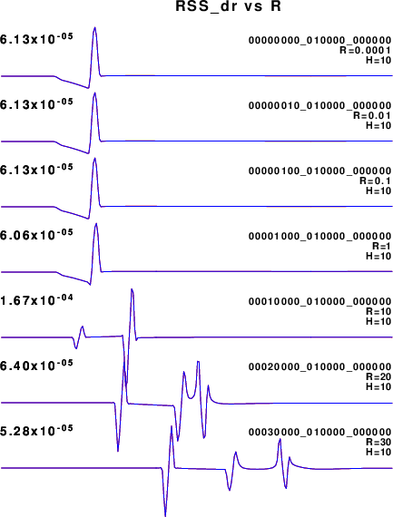
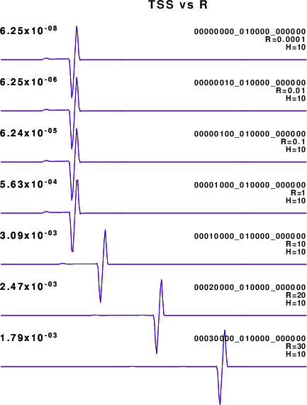
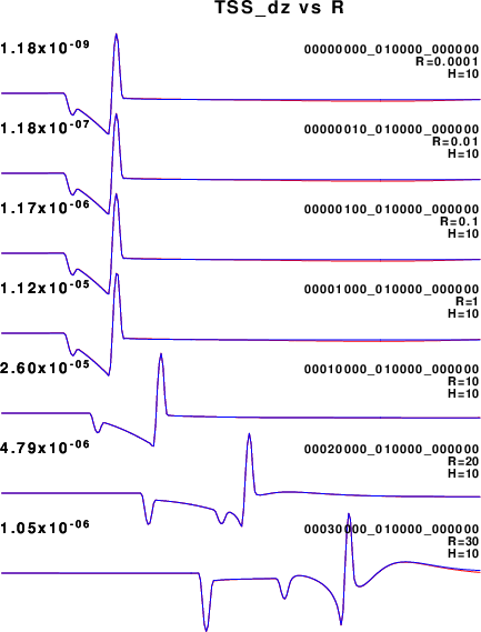
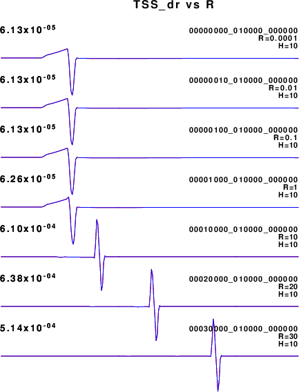
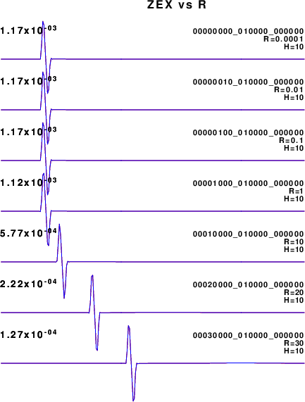
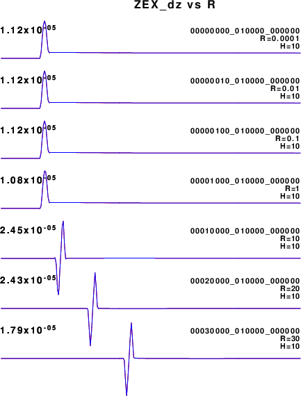
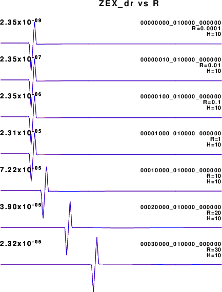
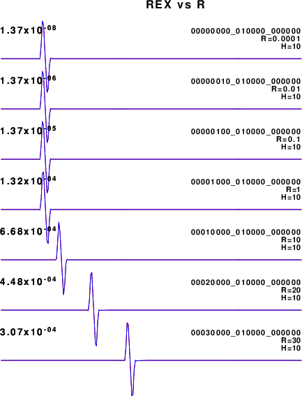
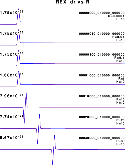
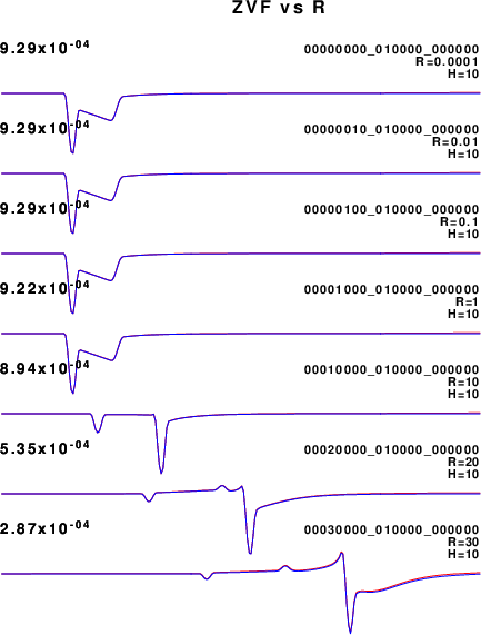
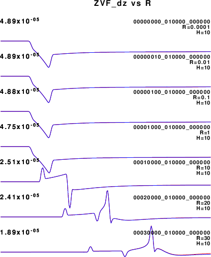
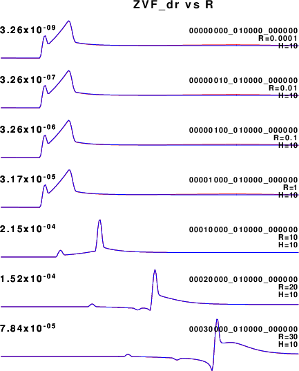
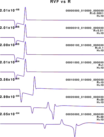
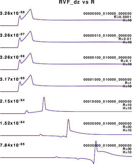
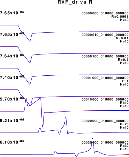
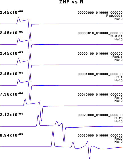
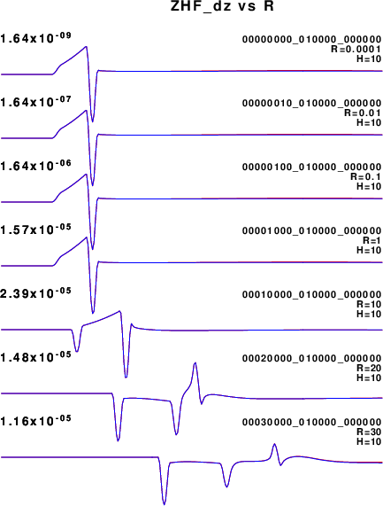
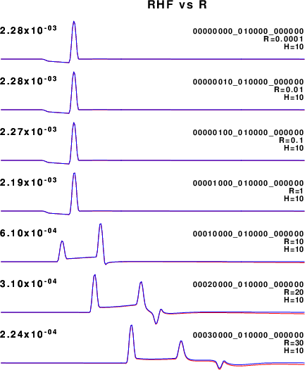
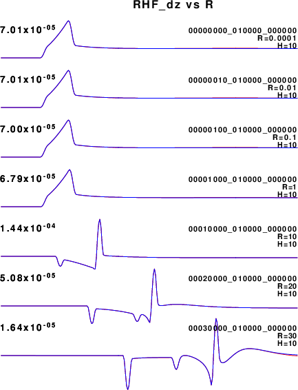
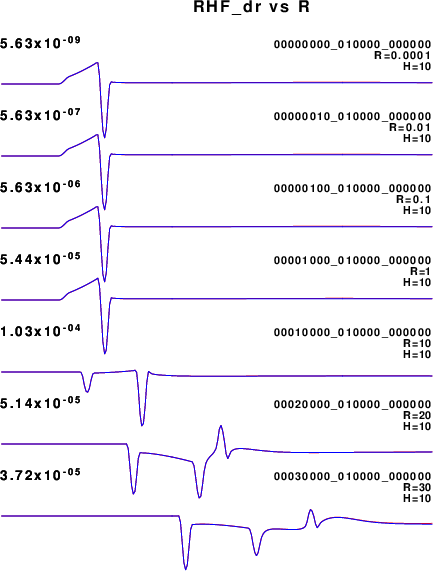
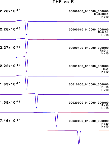
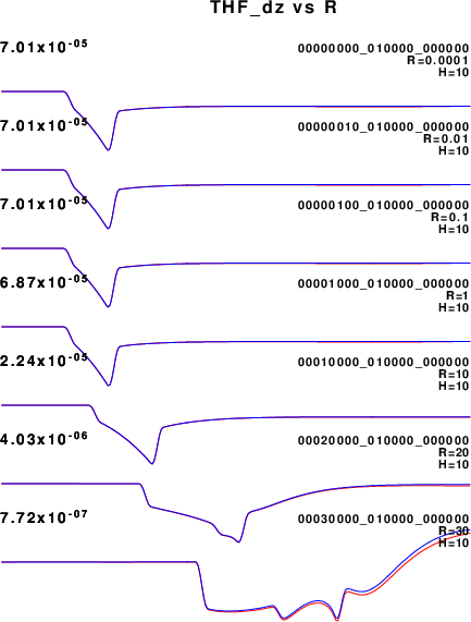
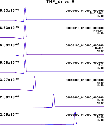
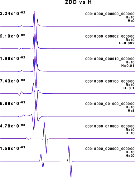
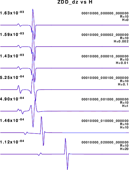
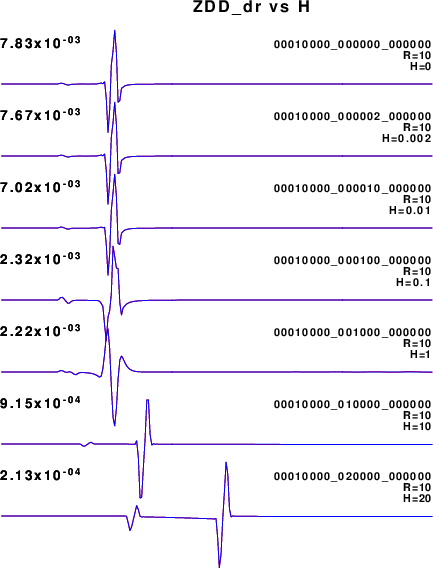
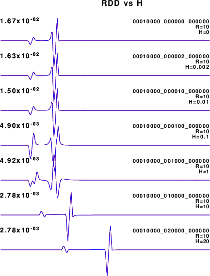
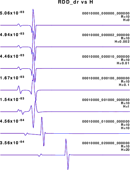
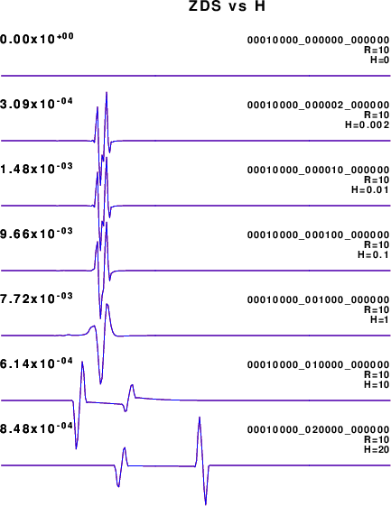
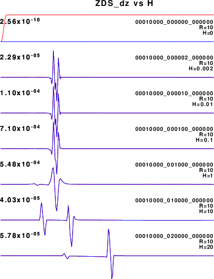
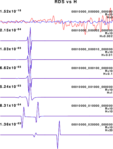
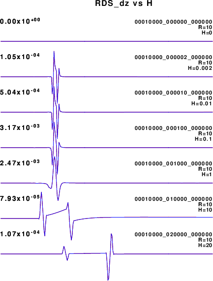
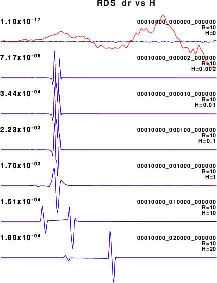
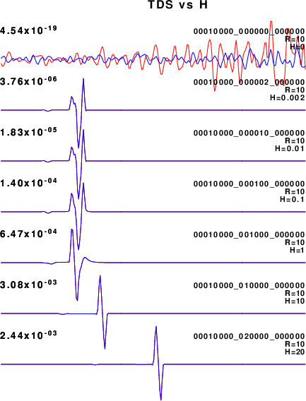
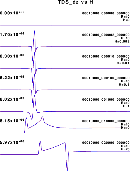
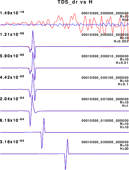
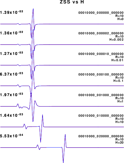
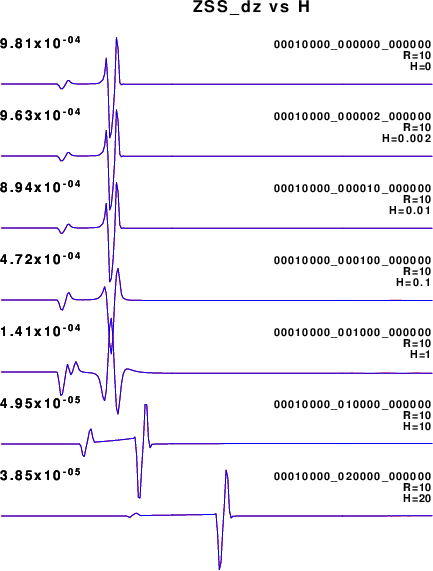
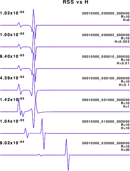
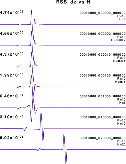
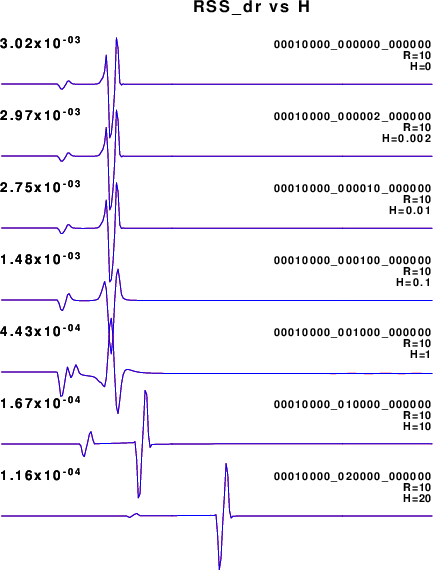
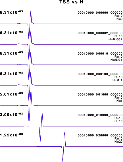
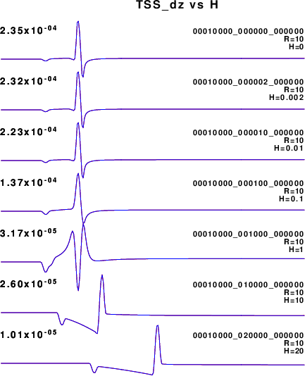
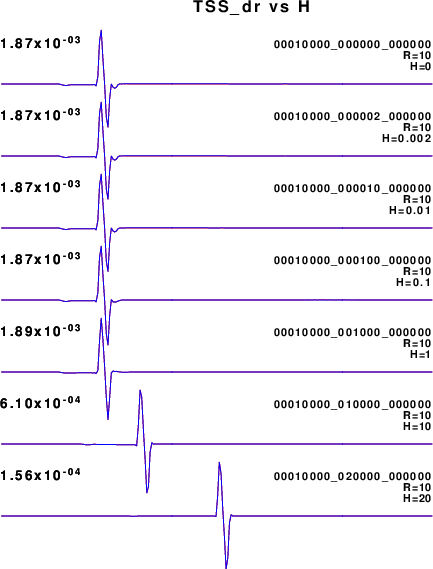
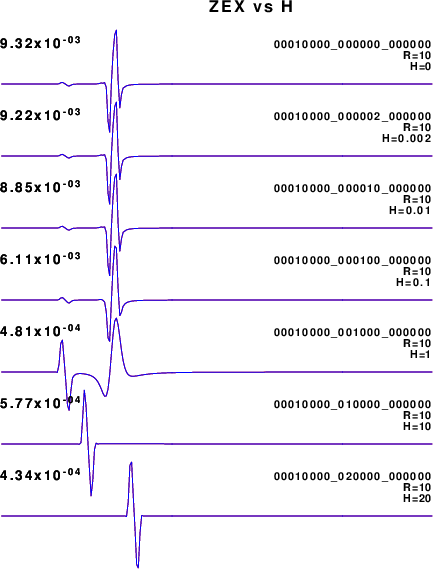
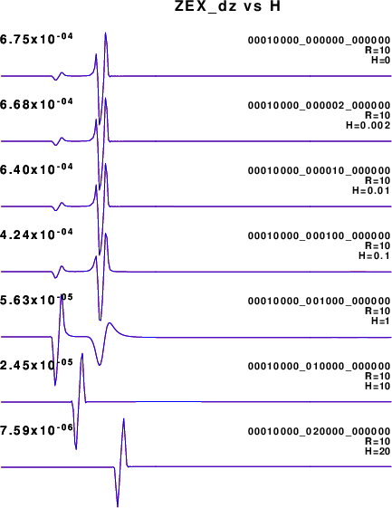
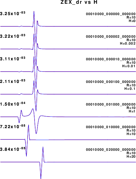
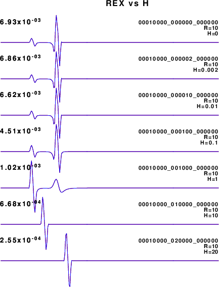
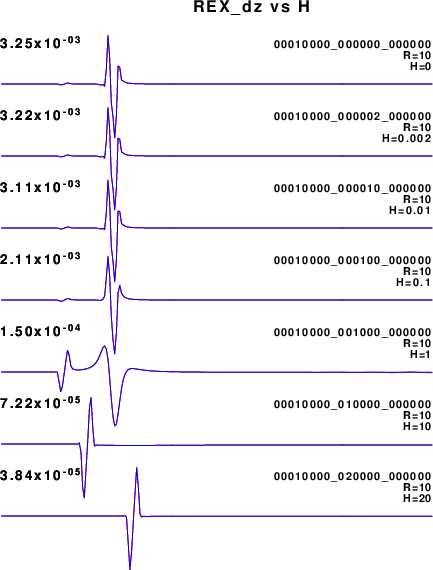
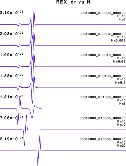
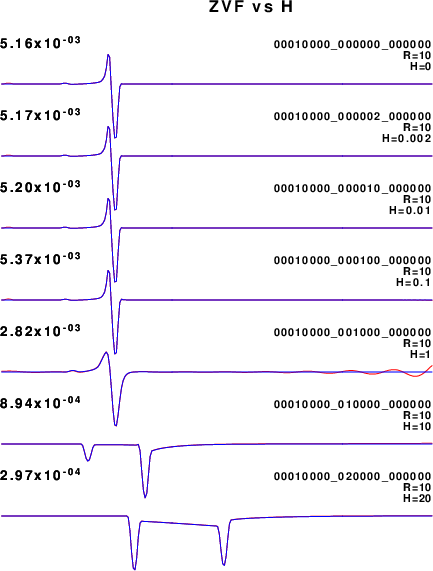
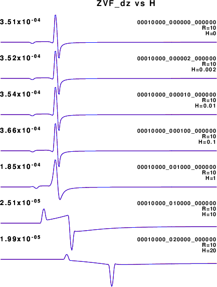
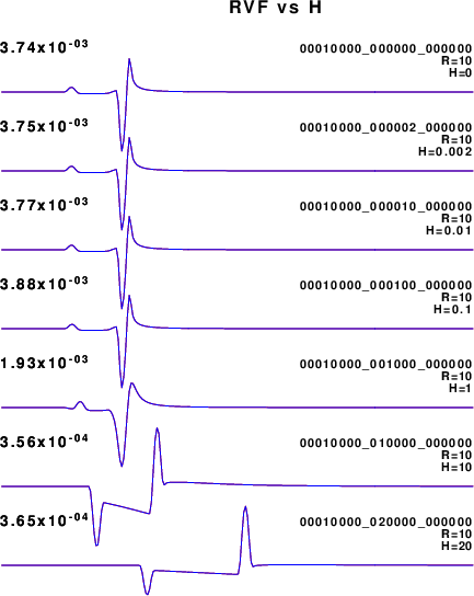
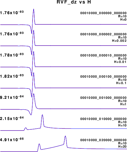
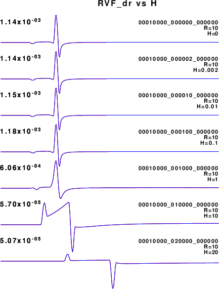
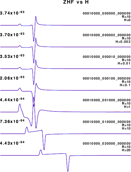
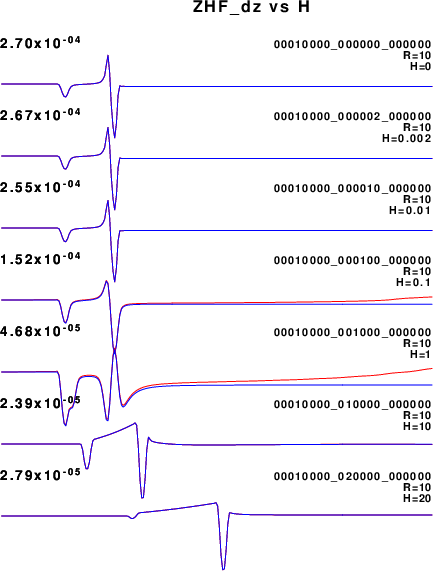
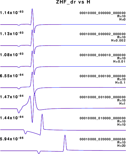
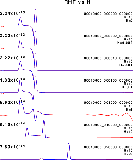
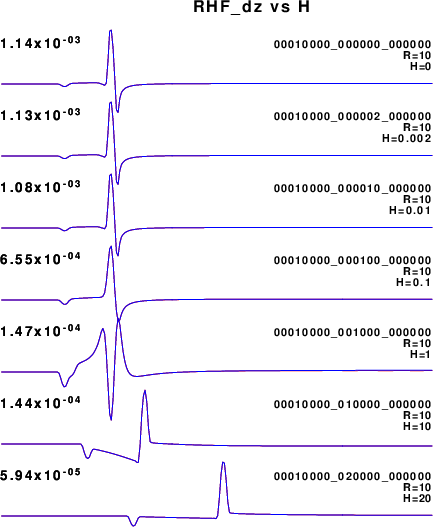
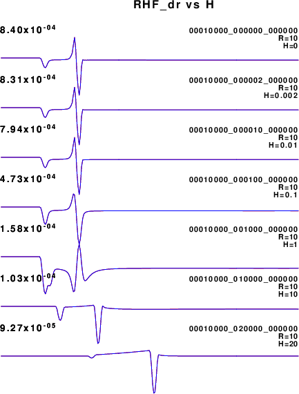
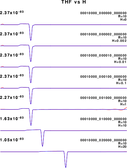
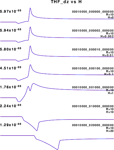
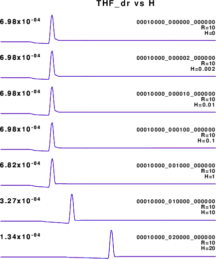
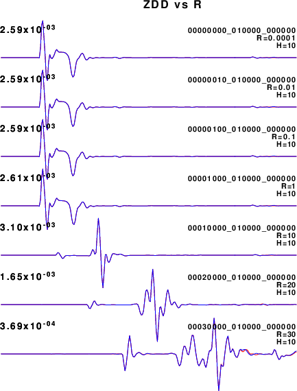
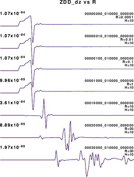
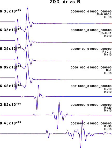
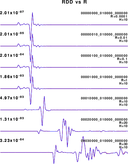
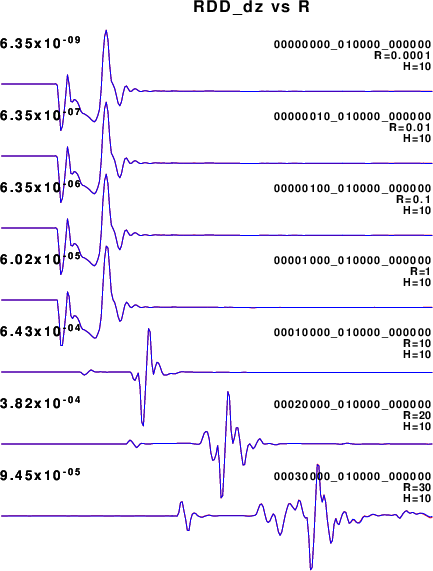
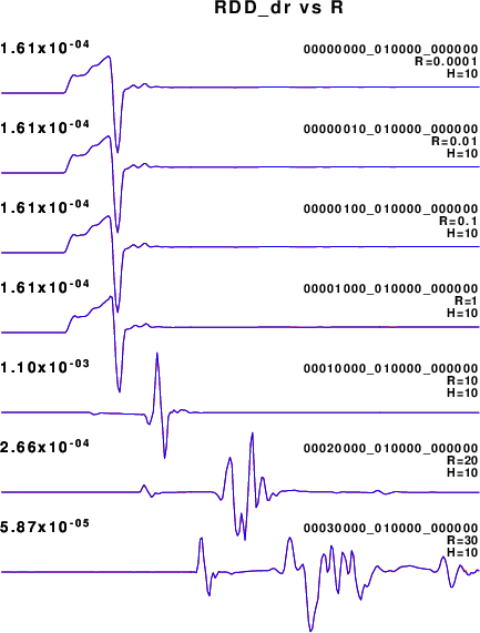
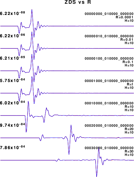
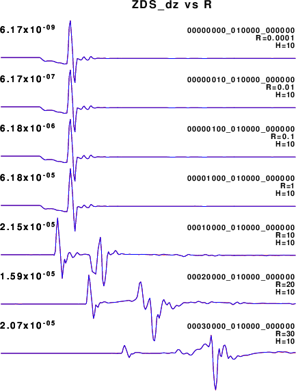
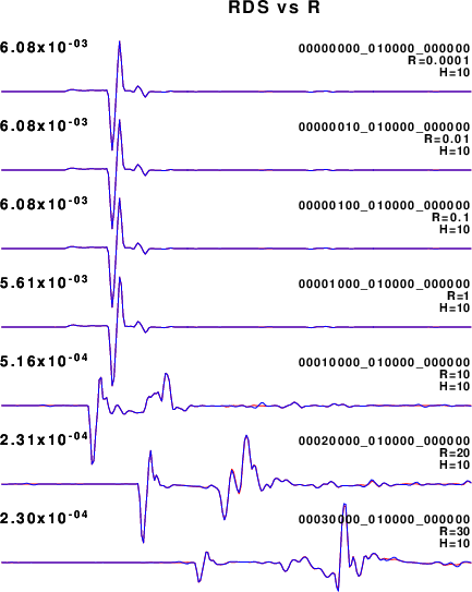
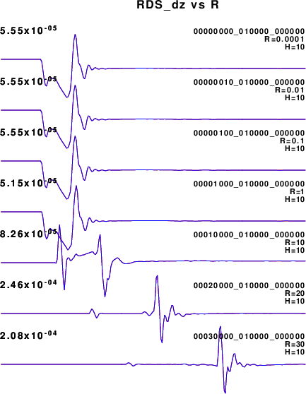
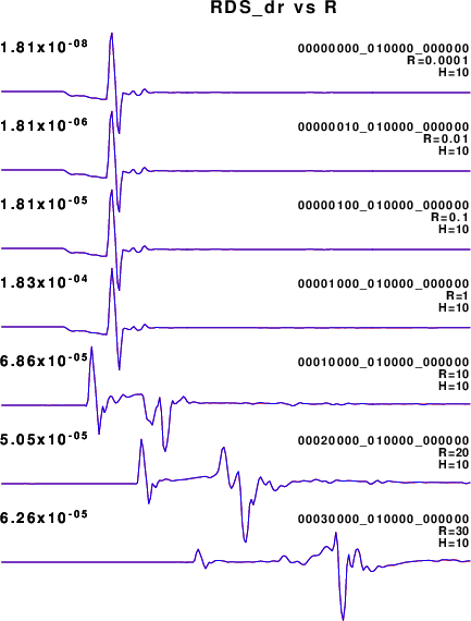
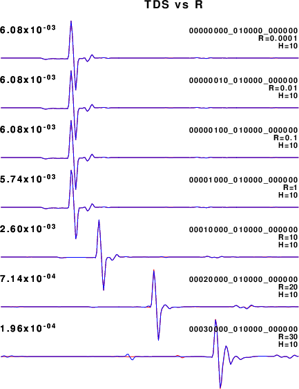
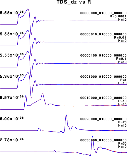
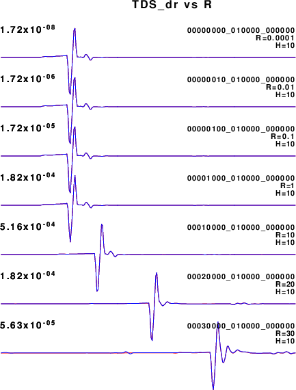
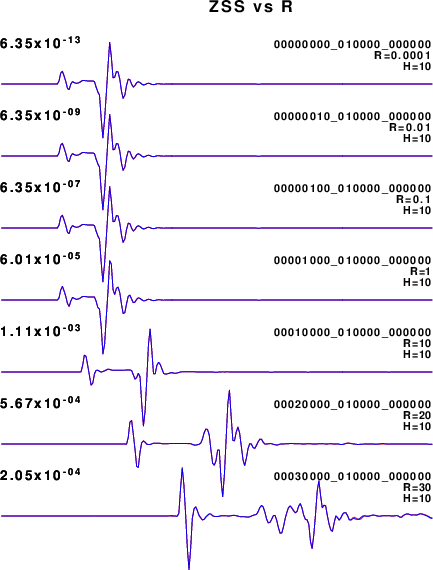
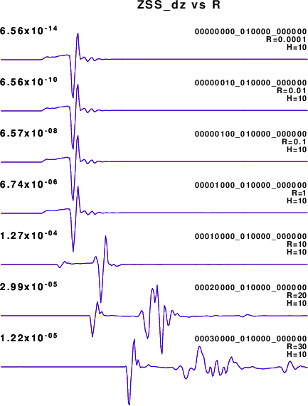
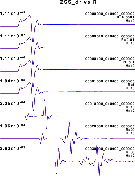
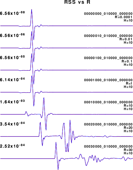
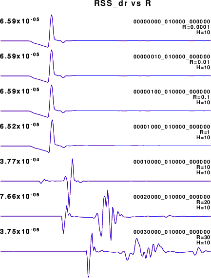
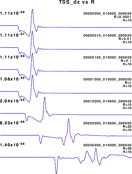
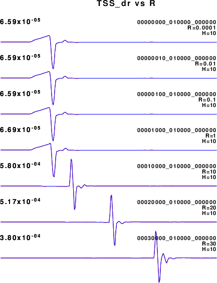
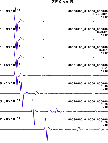
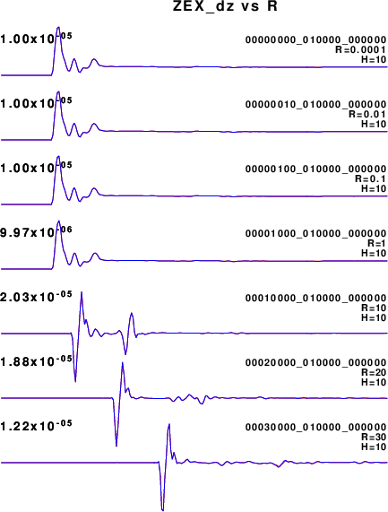
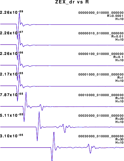
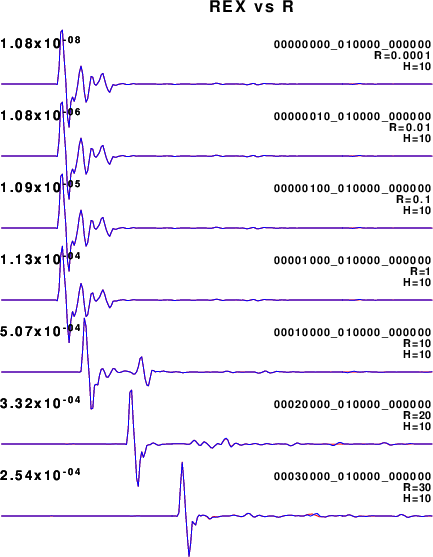
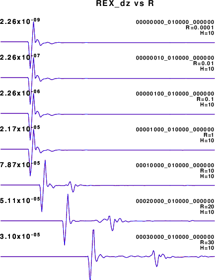
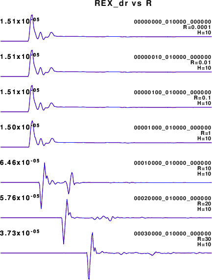
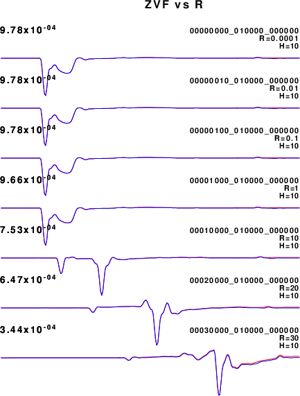
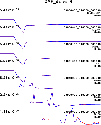
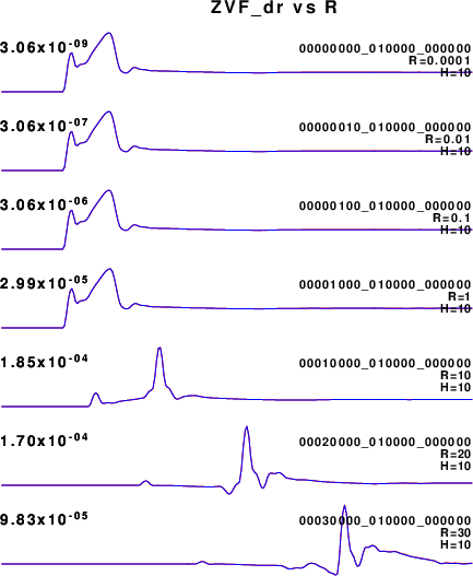
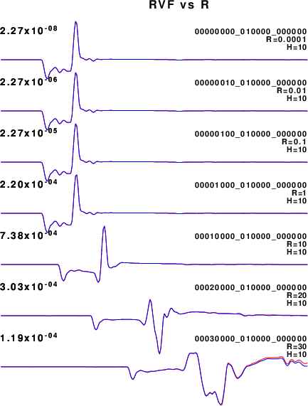
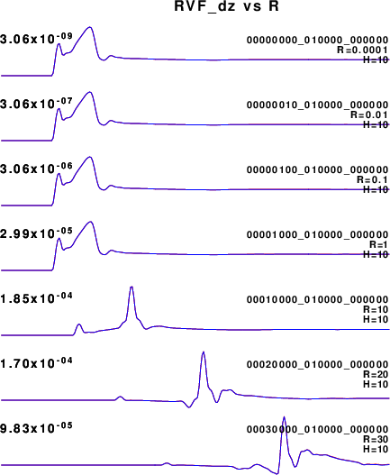
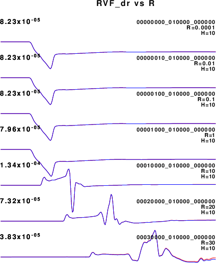
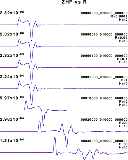
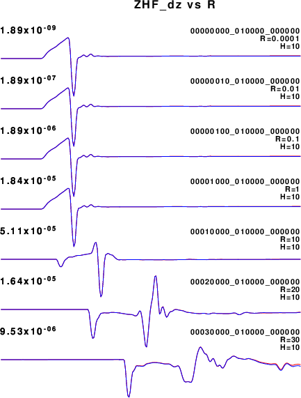
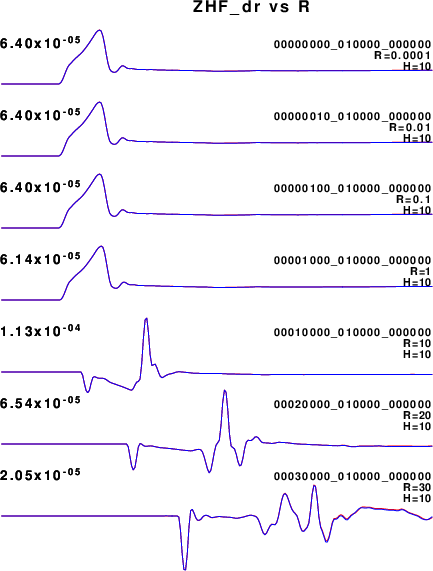
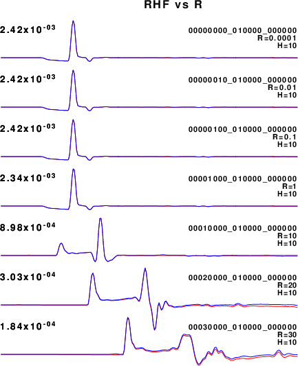
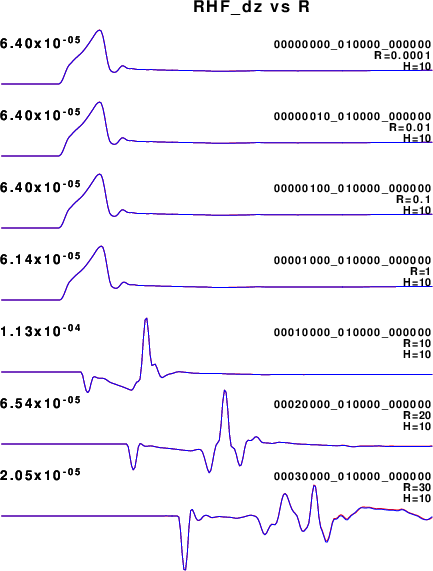
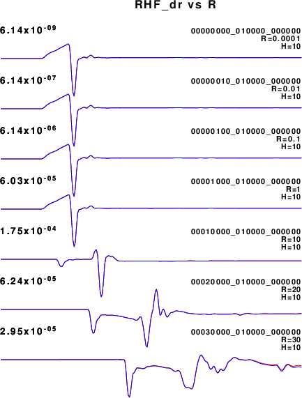
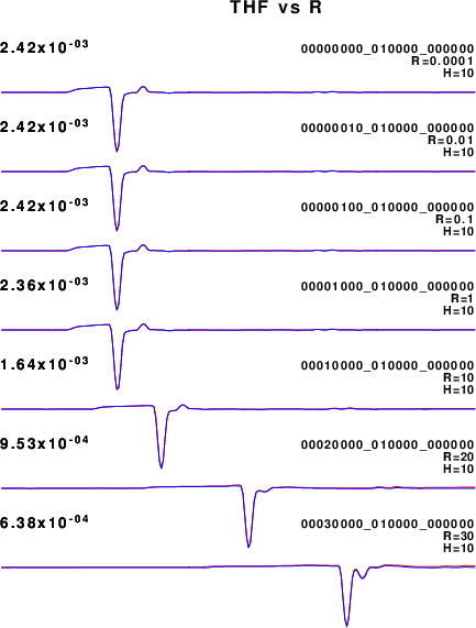
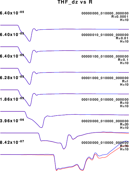
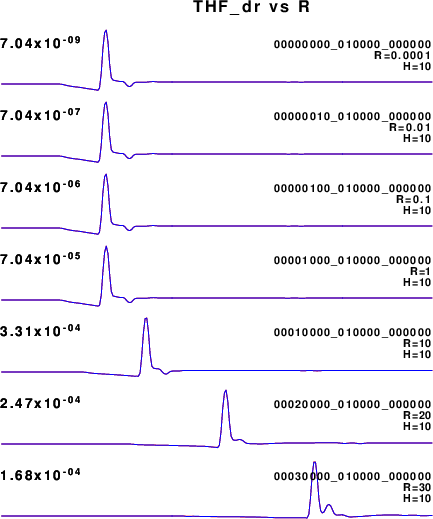
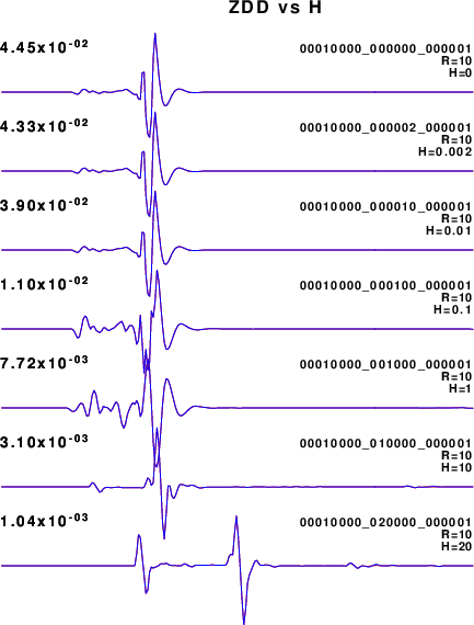
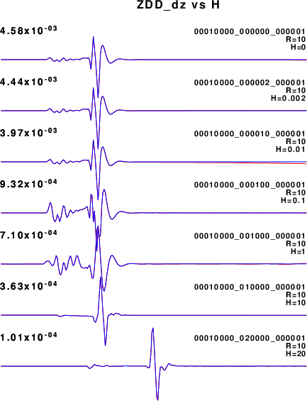
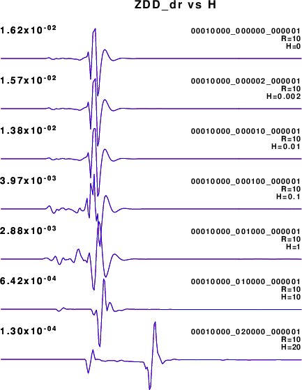
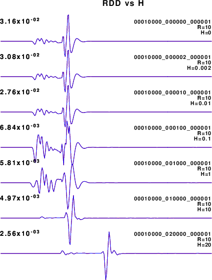
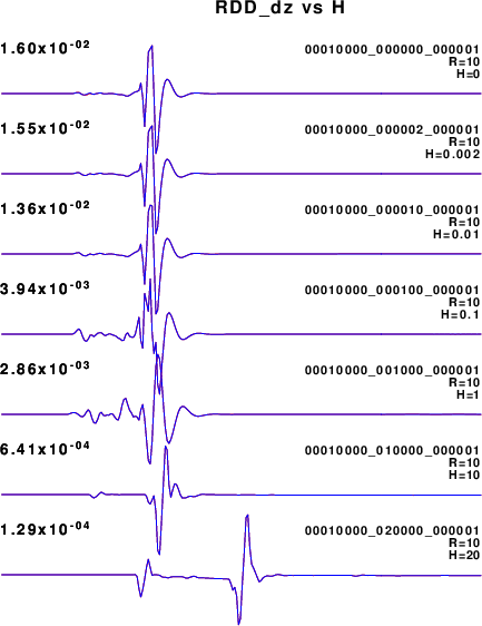
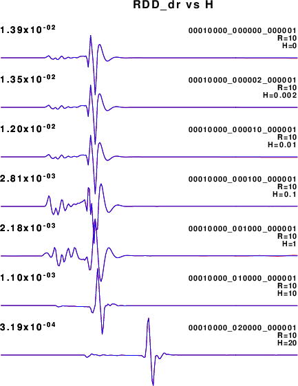
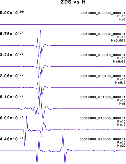
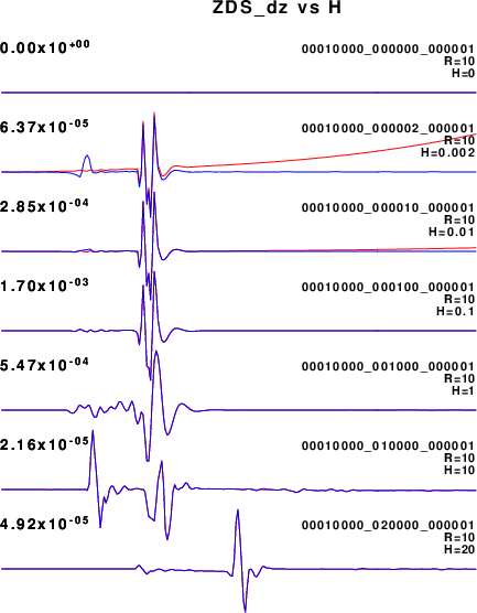
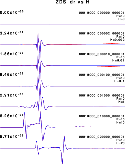
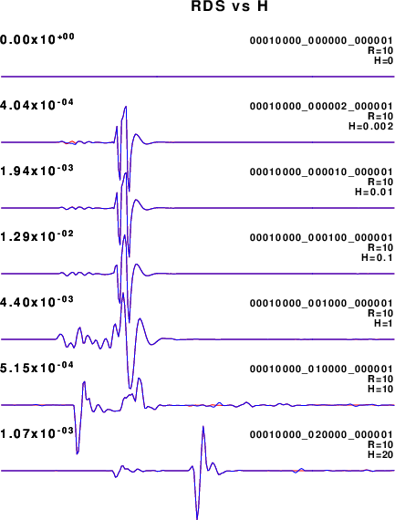
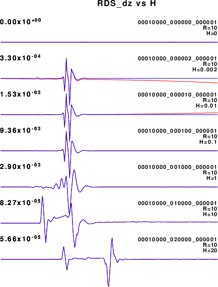
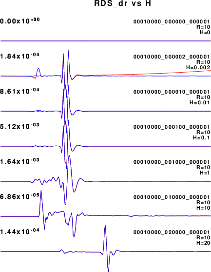
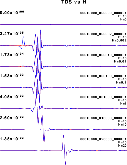
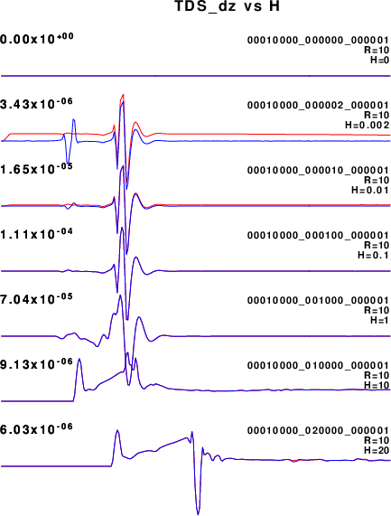
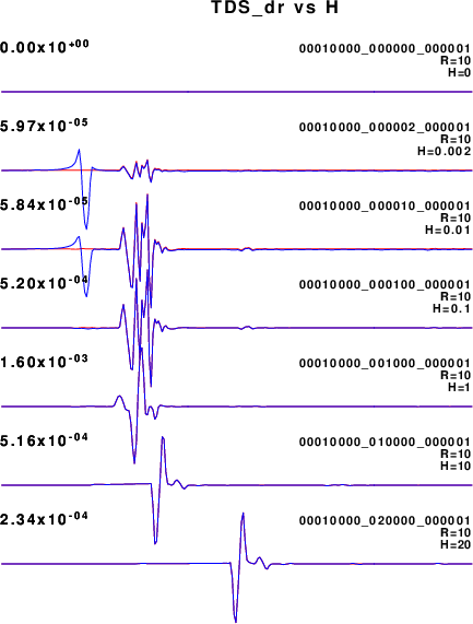
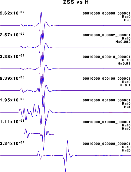
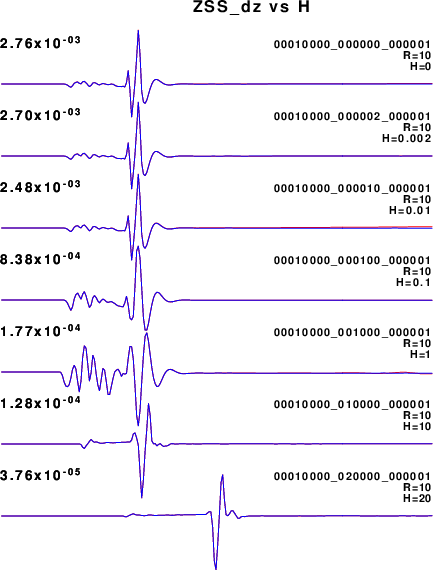
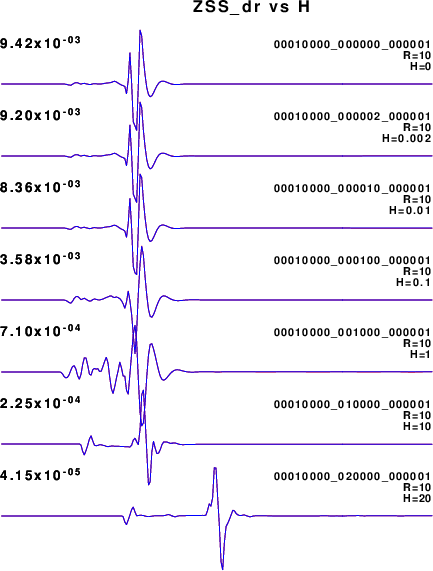
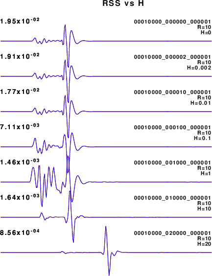
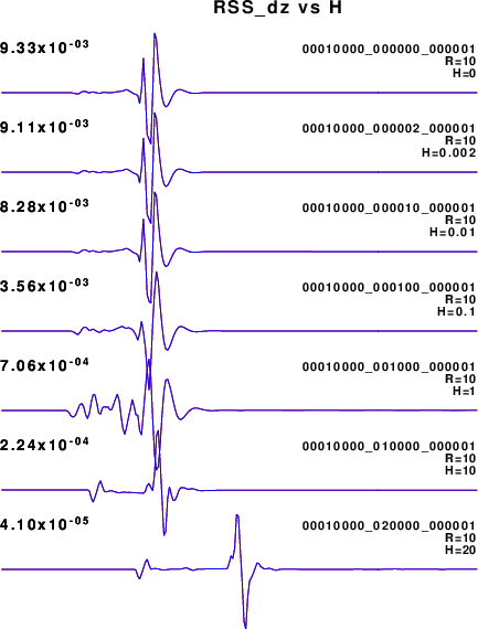
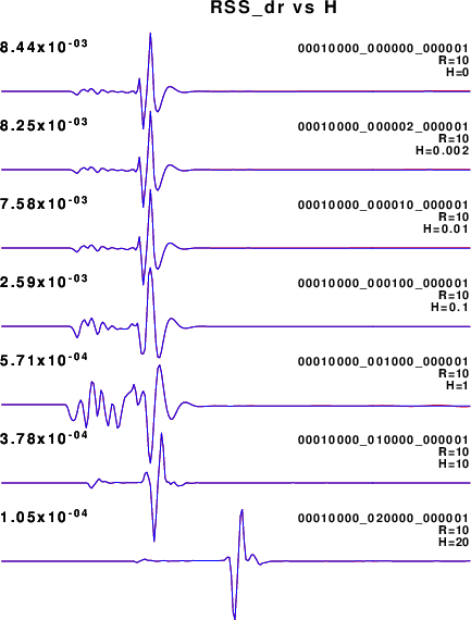
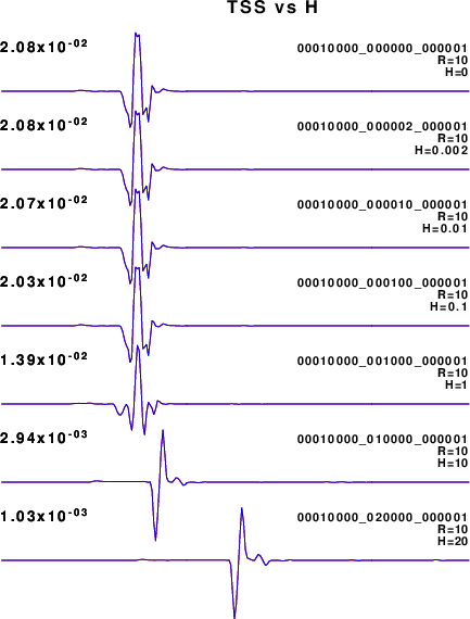
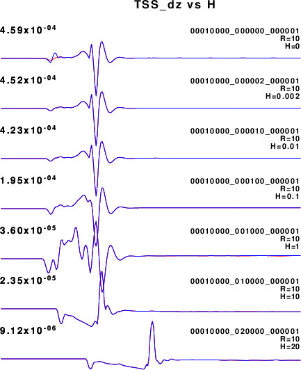
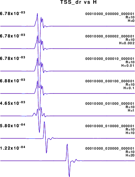
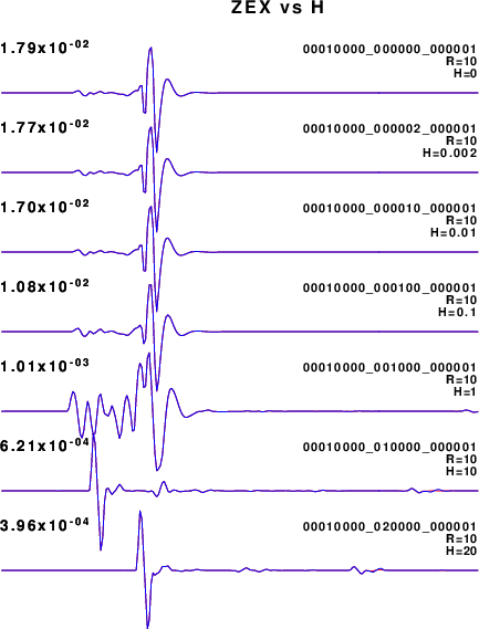
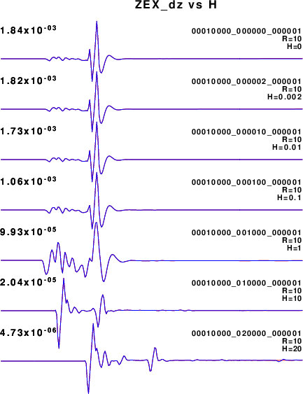
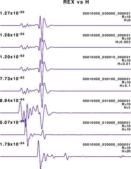
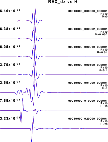
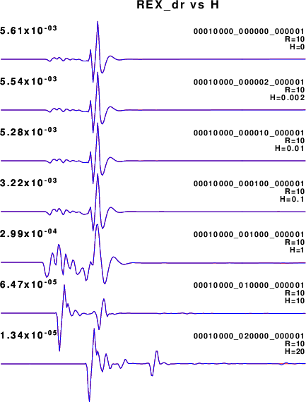
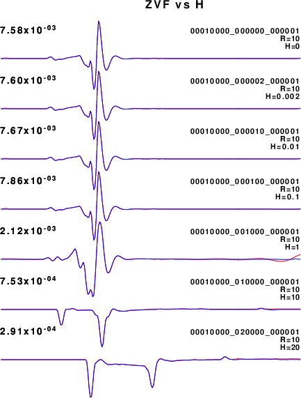
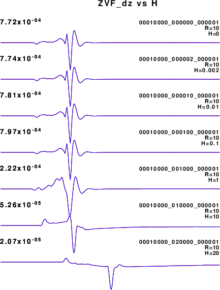
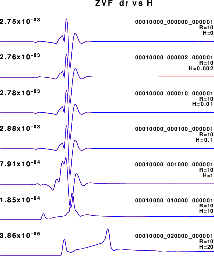
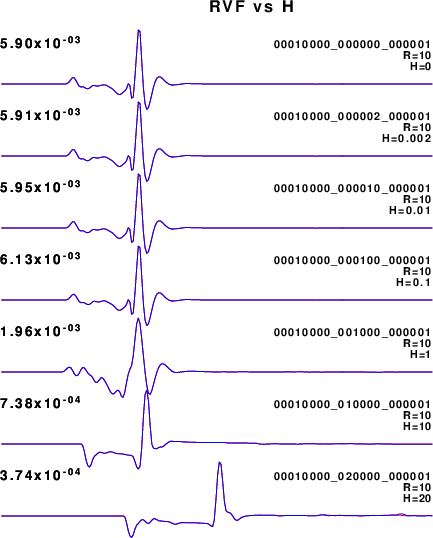
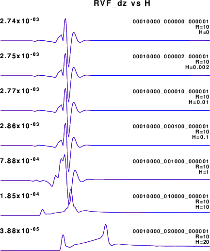
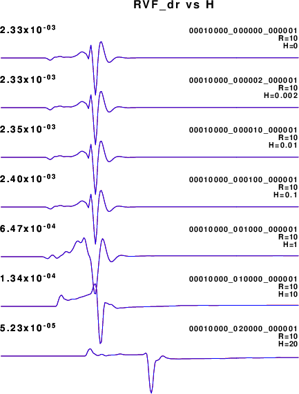
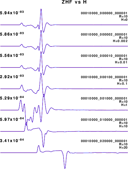
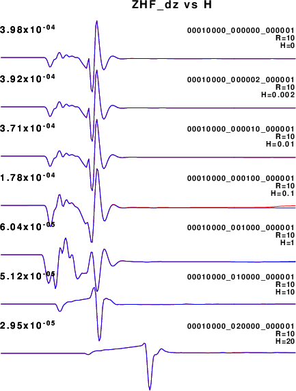
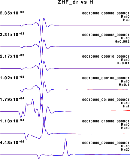
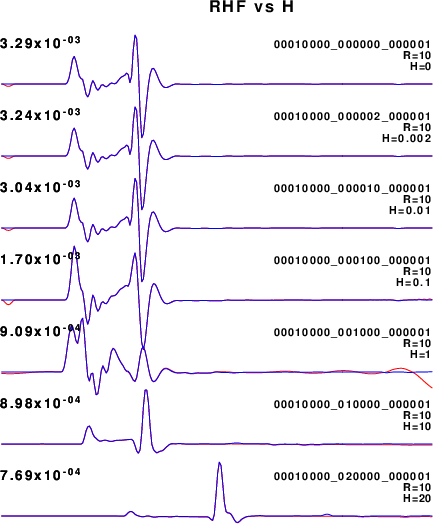
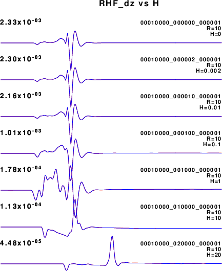
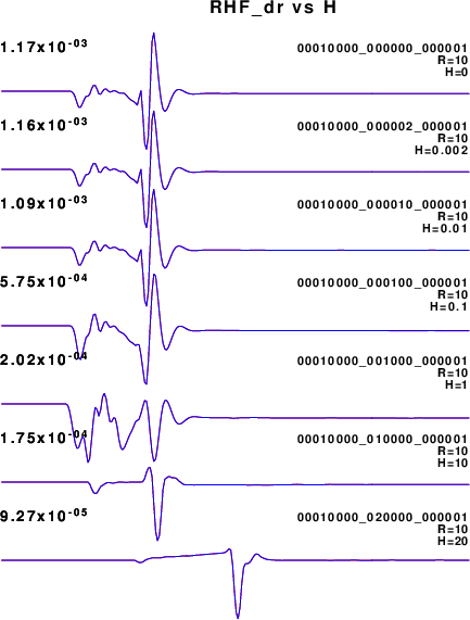
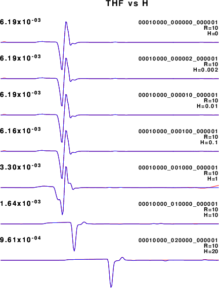
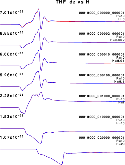
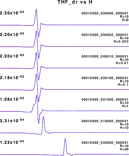
The resulting time series consist of 256 points. The comparison are displayed in figures seen by clicking on the links of the next table. In these figures, the red curve is the true solution from hspec96strain and the blue curve is from sshspec96strain and the traces are overlain. For this wholespace test, the green traces are obtained from hwhole96strain which only requires an inverse Fourier transform and thus does not involve the wavenumber integration. Each comparison is annotated with the peak amplitude, the leading part of the file name which indicates distance, source and receiver depths, the radial distance, as R=0.0001km, and the source depth, as H=10. The receiver depth is 0.0.

Variation of epicentral distance for H=10km Variation of source depth for R=10km

Green's function d /dz d /dr

ZDD d ZDD/dz d ZDD/dr

RDD d RDD/dz d RDD/dr

ZDS d ZDS/dz d ZDS/dr

RDS d RDS/dz d RDS/dr

TDS d TDS/dz d TDS/dr

ZSS d ZSS/dz d ZSS/dr

RSS d RSS/dz d RSS/dr

TSS d TSS/dz d TSS/dr

ZEX d ZEX/dz d ZEX/dr

REX d REX/dz d REX/dr

ZVF d ZVF/dz d ZVF/dr

RVF d RVF/dz d RVF/dr

ZHF d ZHF/dz d ZHF/dr

RHF d RHF/dz d RHF/dr

THF d THF/dz d THF/dr

Green's function d /dz d /dr

ZDD d ZDD/dz d ZDD/dr

RDD d RDD/dz d RDD/dr

ZDS d ZDS/dz d ZDS/dr

RDS d RDS/dz d RDS/dr

TDS d TDS/dz d TDS/dr

ZSS d ZSS/dz d ZSS/dr

RSS d RSS/dz d RSS/dr

TSS d TSS/dz d TSS/dr

ZEX d ZEX/dz d ZEX/dr

REX d REX/dz d REX/dr

ZVF d ZVF/dz d ZVF/dr

RVF d RVF/dz d RVF/dr

ZHF d ZHF/dz d ZHF/dr

RHF d RHF/dz d RHF/dr

THF d THF/dz d THF/dr

For the fixed source depth of H=10, the problems of hspec96strain at R=0 are seen in the d RVF/dr and d TSS/dr.

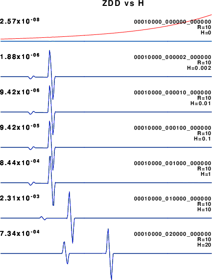
However larger differences are seen for fixed R=10 km as the source depth approaches the receiver depth. The hspec96strain (red curves) is supposed to be zero at H=0 for RDS, TDS, RVF, ZDD, ZEX, ZHF and REX. In most cases the true amplitude may be zero, and the difference reflects numerical error. There are bigger differences in the d/dz of RDD, REX, RHF, RSS, THF, TSS, ZDS. The d/dr of RDS and ZEX show differences.

The conclusion is that the sshspec96strain works well for a wholespace.

Uniform halfspace

The halfspace velocity model, named HALF.mod is created with this shell script:


cat > HALF.mod << EOF
MODEL.01
Simple wholespace model
ISOTROPIC
KGS
FLAT EARTH
1-D
CONSTANT VELOCITY
LINE08
LINE09
LINE10
LINE11
H(KM) VP(KM/S) VS(KM/S) RHO(GM/CC) QP QS ETAP ETAS FREFP FREFS
40.0  6.00       3.5     2.7        0  0  0    0     1     1
EOF

The synthetics are made using the following script which is invoked with the source depth and epicentral distance on the command line. This script differs from the one above in the model used but more importantly in the hprep96 flag -TF which causes the model to be considered as a halfspace with a free surface. [Note that the default of hprep96 is -TF -BH, e.g., free surface at the top and a halfspace at the bottom.] In the comparison the red curve is the true solution from hspec96strain and the blue curve is from sshspec96strain and the traces are overlain.

#!/bin/sh H=$1 R=$2 cat > dfile << EOF ${R} 0.05 256 0 0 EOF hprep96 -M HALF.mod -d dfile -HS ${H} -HR 0 -TF -BH hspec96strain hpulse96strain -TEST1 -V -p -l 2 -FMT 2

#!/bin/sh H=$1 R=$2 cat > dfile << EOF ${R} 0.05 512 0 0 EOF hprep96 -M HALF.mod -d dfile -HS ${H} -HR 0 -TF -BH -XF 8 sshspec96strain hpulse96strain -TEST1 -V -p -l 2 -FMT 2 -HALF

Discussion

Although the solutions require wavenumber integration, the comparisons are excellent for fixed source depth as the epicentral distance increases.

For fixed R, sshspec96strain is much better than hspec96strain as H → 0. The RDS and TDS at H=0 look noisy, but note that the4 amplitudes are very small. The d/dz of ZHF has some noise at about H=1 and the ZDS at H=0 (but is small). Both codes do well for the d/dr.

Layered Halfspace

The final comparison is for a more realistic layered halfspace velocity model, named CUS.mod is created with this shell script:



cat > CUS.mod << EOF
MODEL.01
CUS Model with Q from simple gamma values
ISOTROPIC
KGS
FLAT EARTH
1-D
CONSTANT VELOCITY
LINE08
LINE09
LINE10
LINE11
  H(KM) VP(KM/S) VS(KM/S) RHO(GM/CC)   QP   QS  ETAP  ETAS  FREFP  FREFS
  1.0000  5.0000  2.8900  2.5000 0.172E-02 0.387E-02 0.00  0.00  1.00  1.00 
  9.0000  6.1000  3.5200  2.7300 0.160E-02 0.363E-02 0.00  0.00  1.00  1.00 
 10.0000  6.4000  3.7000  2.8200 0.149E-02 0.336E-02 0.00  0.00  1.00  1.00 
 20.0000  6.7000  3.8700  2.9020 0.000E-04 0.000E-04 0.00  0.00  1.00  1.00 
  0.0000  8.1500  4.7000  3.3640 0.194E-02 0.431E-02 0.00  0.00  1.00  1.00 
EOF

The synthetics are made using the following script which is invoked with the source depth and epicentral distance on the command line.

#!/bin/sh H=$1 R=$2 cat > dfile << EOF ${R} 0.05 256 0 0 EOF hprep96 -M CUS.mod -d dfile -HS ${H} -HR 0 -TF -BH hspec96strain hpulse96strain -TEST1 -V -p -l 2 -FMT 2

#!/bin/sh H=$1 R=$2 cat > dfile << EOF ${R} 0.05 512 0 0 EOF hprep96 -M CUS.mod -d dfile -HS ${H} -HR 0 -TF -BH -XF 8 sshspec96strain hpulse96strain -TEST1 -V -p -l 2 -FMT 2 -HALF

Discussion

Both hspec96strain and sshspec96strain give the same results for H=10 for different values of epicentral distances.

For R=10 as the the source depth varies, sshspec96strain has some artifacts for RDS, TDS, d/dz of ZDS and the d_dr of RDS and TDS The hspec96strain exhibits some long period noise, e.g., RDS_dr and ZDS_dz, while the sshspec96strain has some numerical noise for H=0.002 an H=0.01 for TDS_dr.

3. Summary

This tutorial shows how to evaluate imperfections in the computations. The sshspec96strain works better as the source and receiver positions approach each other.

The sshspec96strain successfully removed some of the low frequency trends for short source-receiver distances.

It seems that the computation for the dip-slip Green's functions, ZDS, RDS and TDS, have more problems when the source and receiver depths become the same. this can be understood from the far-field radiation patterns, for which the P and SH amplitude should be zero for a ray leaving the source horizontally. In addition, there will be problems when the source is at the free surface for these Green's functions.