Location

2013/05/22 17:19:39 35.299 -92.715 5.5 3.5 Arkansas

Arrival Times (from USGS)

Felt Map

Focal Mechanism

USGS/SLU Moment Tensor Solution ENS 2013/05/22 17:19:39:0 35.30 -92.71 5.5 3.5 Arkansas Stations used: AG.FCAR IU.CCM NM.MGMO NM.PBMO NM.PENM NM.UALR TA.TUL1 TA.U40A TA.W39A TA.W41B TA.X40A Filtering commands used: hp c 0.03 n 3 lp c 0.10 n 3 Best Fitting Double Couple Mo = 1.48e+21 dyne-cm Mw = 3.38 Z = 2 km Plane Strike Dip Rake NP1 182 71 -159 NP2 85 70 -20 Principal Axes: Axis Value Plunge Azimuth T 1.48e+21 1 313 N 0.00e+00 62 222 P -1.48e+21 28 44 Moment Tensor: (dyne-cm) Component Value Mxx 9.59e+19 Mxy -1.31e+21 Mxz -4.27e+20 Myy 2.29e+20 Myz -4.40e+20 Mzz -3.25e+20 #######------- ##########------------ ###########---------------- T ##########------------------ # ##########------------ ----- ##############------------- P ------ ###############------------- ------- ################------------------------ ################------------------------ ################-------------------------- ################-------------------------# ################----------------------#### --##############-----------------######### -------########---------################ ---------------######################### ---------------####################### --------------###################### -------------##################### -----------################### -----------################# ---------############# -----######### Global CMT Convention Moment Tensor: R T P -3.25e+20 -4.27e+20 4.40e+20 -4.27e+20 9.59e+19 1.31e+21 4.40e+20 1.31e+21 2.29e+20 Details of the solution is found at http://www.eas.slu.edu/Earthquake_Center/MECH.NA/20130522171939/index.html

Preferred Solution

The preferred solution from an analysis of the surface-wave spectral amplitude radiation pattern, waveform inversion and first motion observations is

      STK = 85
      DIP = 70
     RAKE = -20
       MW = 3.38
       HS = 2.0

The waveform inversion is preferred.

Moment Tensor Comparison

The following compares this source inversion to others

SLU

USGS/SLU Moment Tensor Solution ENS 2013/05/22 17:19:39:0 35.30 -92.71 5.5 3.5 Arkansas Stations used: AG.FCAR IU.CCM NM.MGMO NM.PBMO NM.PENM NM.UALR TA.TUL1 TA.U40A TA.W39A TA.W41B TA.X40A Filtering commands used: hp c 0.03 n 3 lp c 0.10 n 3 Best Fitting Double Couple Mo = 1.48e+21 dyne-cm Mw = 3.38 Z = 2 km Plane Strike Dip Rake NP1 182 71 -159 NP2 85 70 -20 Principal Axes: Axis Value Plunge Azimuth T 1.48e+21 1 313 N 0.00e+00 62 222 P -1.48e+21 28 44 Moment Tensor: (dyne-cm) Component Value Mxx 9.59e+19 Mxy -1.31e+21 Mxz -4.27e+20 Myy 2.29e+20 Myz -4.40e+20 Mzz -3.25e+20 #######------- ##########------------ ###########---------------- T ##########------------------ # ##########------------ ----- ##############------------- P ------ ###############------------- ------- ################------------------------ ################------------------------ ################-------------------------- ################-------------------------# ################----------------------#### --##############-----------------######### -------########---------################ ---------------######################### ---------------####################### --------------###################### -------------##################### -----------################### -----------################# ---------############# -----######### Global CMT Convention Moment Tensor: R T P -3.25e+20 -4.27e+20 4.40e+20 -4.27e+20 9.59e+19 1.31e+21 4.40e+20 1.31e+21 2.29e+20 Details of the solution is found at http://www.eas.slu.edu/Earthquake_Center/MECH.NA/20130522171939/index.html

Waveform Inversion

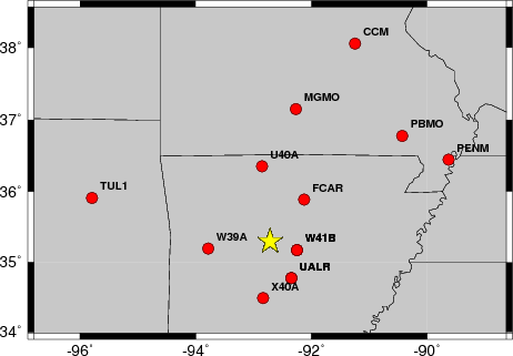
The focal mechanism was determined using broadband seismic waveforms. The location of the event and the and stations used for the waveform inversion are shown in the next figure.

Location of broadband stations used for waveform inversion

The program wvfgrd96 was used with good traces observed at short distance to determine the focal mechanism, depth and seismic moment. This technique requires a high quality signal and well determined velocity model for the Green functions. To the extent that these are the quality data, this type of mechanism should be preferred over the radiation pattern technique which requires the separate step of defining the pressure and tension quadrants and the correct strike.

The observed and predicted traces are filtered using the following gsac commands:

hp c 0.03 n 3
lp c 0.10 n 3

The results of this grid search from 0.5 to 19 km depth are as follow:

           DEPTH  STK   DIP  RAKE   MW    FIT
WVFGRD96    0.5    90    75    -5   3.30 0.5134
WVFGRD96    1.0    90    75   -10   3.33 0.5374
WVFGRD96    2.0    85    70   -20   3.38 0.5615
WVFGRD96    3.0    90    70   -15   3.40 0.5588
WVFGRD96    4.0    90    70   -15   3.41 0.5489
WVFGRD96    5.0    90    70   -15   3.41 0.5357
WVFGRD96    6.0   270    85    25   3.43 0.5339
WVFGRD96    7.0   270    70    10   3.43 0.5351
WVFGRD96    8.0   275    80    25   3.45 0.5361
WVFGRD96    9.0   275    80    25   3.46 0.5369
WVFGRD96   10.0   275    80    25   3.47 0.5372
WVFGRD96   11.0   275    80    25   3.48 0.5343
WVFGRD96   12.0   275    80    25   3.49 0.5317
WVFGRD96   13.0   275    80    25   3.50 0.5296
WVFGRD96   14.0   275    80    25   3.51 0.5268
WVFGRD96   15.0   275    80    25   3.52 0.5227
WVFGRD96   16.0   270    70    10   3.51 0.5184
WVFGRD96   17.0   270    70    10   3.52 0.5155
WVFGRD96   18.0   270    70    10   3.52 0.5121
WVFGRD96   19.0   270    70    10   3.53 0.5079
WVFGRD96   20.0   270    65    10   3.55 0.5046
WVFGRD96   21.0   275    60    15   3.57 0.5012
WVFGRD96   22.0   275    60    15   3.57 0.4973
WVFGRD96   23.0   270    60    10   3.57 0.4948
WVFGRD96   24.0   270    60     5   3.58 0.4926
WVFGRD96   25.0   270    60    10   3.59 0.4895
WVFGRD96   26.0   270    55    10   3.60 0.4883
WVFGRD96   27.0   270    55    10   3.61 0.4855
WVFGRD96   28.0   270    55    10   3.61 0.4839
WVFGRD96   29.0   260    65   -20   3.59 0.4804

The best solution is

WVFGRD96    2.0    85    70   -20   3.38 0.5615

The mechanism correspond to the best fit is

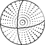
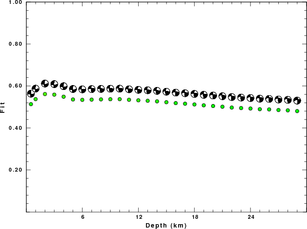
Figure 1. Waveform inversion focal mechanism

The best fit as a function of depth is given in the following figure:

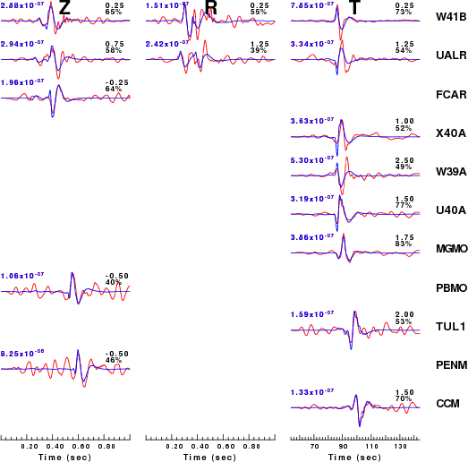
Figure 2. Depth sensitivity for waveform mechanism

The comparison of the observed and predicted waveforms is given in the next figure. The red traces are the observed and the blue are the predicted. Each observed-predicted component is plotted to the same scale and peak amplitudes are indicated by the numbers to the left of each trace. A pair of numbers is given in black at the right of each predicted traces. The upper number it the time shift required for maximum correlation between the observed and predicted traces. This time shift is required because the synthetics are not computed at exactly the same distance as the observed and because the velocity model used in the predictions may not be perfect. A positive time shift indicates that the prediction is too fast and should be delayed to match the observed trace (shift to the right in this figure). A negative value indicates that the prediction is too slow. The lower number gives the percentage of variance reduction to characterize the individual goodness of fit (100% indicates a perfect fit).

The bandpass filter used in the processing and for the display was

hp c 0.03 n 3
lp c 0.10 n 3

The plots below start 30 seconds before the theoretical S arrival and continue until 60 seconds after the theoretical S arrival.

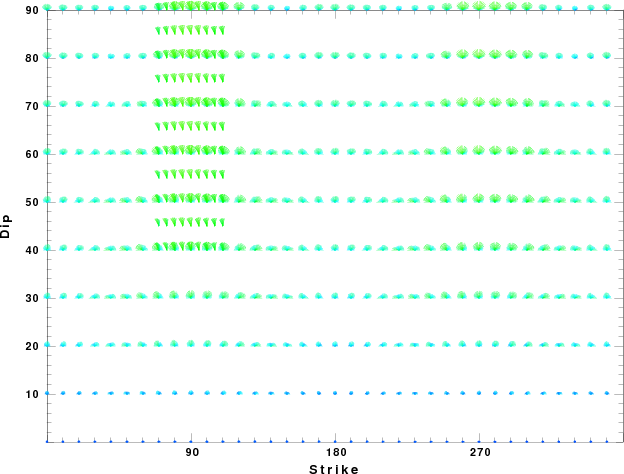
Figure 3. Waveform comparison for selected depth

Focal mechanism sensitivity at the preferred depth. The red color indicates a very good fit to thewavefroms. Each solution is plotted as a vector at a given value of strike and dip with the angle of the vector representing the rake angle, measured, with respect to the upward vertical (N) in the figure.

A check on the assumed source location is possible by looking at the time shifts between the observed and predicted traces. The time shifts for waveform matching arise for several reasons:

The origin time and epicentral distance are incorrect
The velocity model used for the inversion is incorrect
The velocity model used to define the P-arrival time is not the same as the velocity model used for the waveform inversion (assuming that the initial trace alignment is based on the P arrival time)

Assuming only a mislocation, the time shifts are fit to a functional form:

 Time_shift = A + B cos Azimuth + C Sin Azimuth

The time shifts for this inversion lead to the next figure:

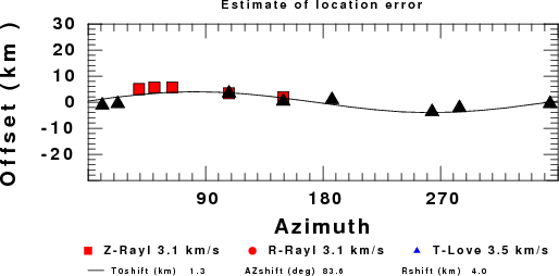
The derived shift in origin time and epicentral coordinates are given at the bottom of the figure.

Discussion

Thanks also to the many seismic network operators whose dedication make this effort possible: University of Alaska, University of Washington, Oregon State University, University of Utah, Montana Bureas of Mines, UC Berkely, Caltech, UC San Diego, Saint Louis University, University of Memphis, Lamont Doherty Earth Observatory, the IRIS stations and the Transportable Array of EarthScope.

Velocity Model

The WUS used for the waveform synthetic seismograms and for the surface wave eigenfunctions and dispersion is as follows:

MODEL.01
Model after     8 iterations
ISOTROPIC
KGS
FLAT EARTH
1-D
CONSTANT VELOCITY
LINE08
LINE09
LINE10
LINE11
      H(KM)   VP(KM/S)   VS(KM/S) RHO(GM/CC)         QP         QS       ETAP       ETAS      FREFP      FREFS
     1.9000     3.4065     2.0089     2.2150  0.302E-02  0.679E-02   0.00       0.00       1.00       1.00    
     6.1000     5.5445     3.2953     2.6089  0.349E-02  0.784E-02   0.00       0.00       1.00       1.00    
    13.0000     6.2708     3.7396     2.7812  0.212E-02  0.476E-02   0.00       0.00       1.00       1.00    
    19.0000     6.4075     3.7680     2.8223  0.111E-02  0.249E-02   0.00       0.00       1.00       1.00    
     0.0000     7.9000     4.6200     3.2760  0.164E-10  0.370E-10   0.00       0.00       1.00       1.00

Quality Control

Here we tabulate the reasons for not using certain digital data sets

The following stations did not have a valid response files:

DATE=Wed May 22 15:53:05 CDT 2013

Last Changed 2013/05/22