Location
Location ANSS
The ANSS event ID is nc40204628 and the event page is at
https://earthquake.usgs.gov/earthquakes/eventpage/nc40204628/executive.
2007/10/31 03:04:54 37.434 -121.774 9.7 5.45 California
Focal Mechanism
 USGS/SLU Moment Tensor Solution
 ENS  2007/10/31 03:04:54:0  37.43 -121.77   9.7 5.4 California

 Stations used:
   BK.BDM BK.CMB BK.CVS BK.FARB BK.HOPS BK.JCC BK.JRSC BK.KCC
   BK.MCCM BK.MNRC BK.ORV BK.PKD BK.SAO BK.WDC BK.WENL BK.YBH
   CI.CHF CI.CWC CI.DEC CI.DJJ CI.EDW2 CI.FUR CI.GRA CI.GSC
   CI.ISA CI.LRL CI.MLAC CI.MPM CI.MPP CI.MWC CI.PASC CI.PHL
   CI.RCT CI.SBC CI.SCZ2 CI.SHO CI.SLA CI.SMM CI.TIN CI.VCS
   CI.VES G.SCZ IM.NV31 LB.BMN LB.TPH NN.PAH NN.WCN TA.LAVA
   TA.M02C TA.M07A TA.M08A TA.N02C TA.N06A TA.N07B TA.N08A
   TA.N09A TA.O01C TA.O06A TA.O07A TA.O08A TA.P06A TA.P07A
   TA.P09A TA.Q07A TA.Q08A TA.Q09A TA.Q10A TA.R04C TA.R06C
   TA.R08A TA.R09A TA.R10A TA.S05C TA.S09A TA.S10A TA.S11A
   TA.T06C TA.U04C TA.U05C TA.U10A TA.V03C US.TPNV XQ.ME05
   XQ.ME34 XQ.ME36 XQ.ME43 XQ.ME44 XQ.ME45 XQ.ME46 XQ.ME47
   XQ.ME48 XQ.ME49 XQ.ME50 XQ.ME53 XQ.ME54 XQ.ME81 XQ.ME84
   XQ.ME92 XQ.ME93

 Filtering commands used:
   cut o DIST/3.3 -40 o DIST/3.3 +50
   rtr
   taper w 0.1
   hp c 0.03 n 3
   lp c 0.06 n 3

 Best Fitting Double Couple
  Mo = 2.02e+24 dyne-cm
  Mw = 5.47
  Z  = 16 km
  Plane   Strike  Dip  Rake
   NP1      235    80   -15
   NP2      328    75   -170
  Principal Axes:
   Axis    Value   Plunge  Azimuth
    T   2.02e+24      3     282
    N   0.00e+00     72      22
    P  -2.02e+24     18     191

 Moment Tensor: (dyne-cm)
    Component   Value
       Mxx    -1.68e+24
       Mxy    -7.41e+23
       Mxz     5.96e+23
       Myy     1.86e+24
       Myz    -4.24e+21
       Mzz    -1.79e+23


                     --------------
                 ----------------------
              ######----------------------
             #########---------------------
           #############---------------------
          ###############---------------######
         ##################----------##########
          ##################-----###############
        T ###################-##################
          ##################---##################
       ##################-------#################
       ###############-----------################
       #############--------------###############
        ##########-----------------#############
        ########--------------------############
         #####-----------------------##########
          ##-------------------------#########
           ---------------------------#######
             -------------------------#####
              ---------   -------------###
                 ------ P -------------
                     --   ---------


 Global CMT Convention Moment Tensor:
      R          T          P
 -1.79e+23   5.96e+23   4.24e+21
  5.96e+23  -1.68e+24   7.41e+23
  4.24e+21   7.41e+23   1.86e+24


Details of the solution is found at

http://www.eas.slu.edu/eqc/eqc_mt/MECH.NA/20071031030454/index.html
|
Preferred Solution
The preferred solution from an analysis of the surface-wave spectral amplitude radiation pattern, waveform inversion or first motion observations is
      STK = 235
      DIP = 80
     RAKE = -15
       MW = 5.47
       HS = 16.0
The NDK file is 20071031030454.ndk
The waveform inversion is preferred.
Moment Tensor Comparison
The following compares this source inversion to those provided by others. The purpose is to look for major differences and also to note slight differences that might be inherent to the processing procedure. For completeness the USGS/SLU solution is repeated from above.
| SLU |
GCMT |
UCB |
 USGS/SLU Moment Tensor Solution
 ENS  2007/10/31 03:04:54:0  37.43 -121.77   9.7 5.4 California

 Stations used:
   BK.BDM BK.CMB BK.CVS BK.FARB BK.HOPS BK.JCC BK.JRSC BK.KCC
   BK.MCCM BK.MNRC BK.ORV BK.PKD BK.SAO BK.WDC BK.WENL BK.YBH
   CI.CHF CI.CWC CI.DEC CI.DJJ CI.EDW2 CI.FUR CI.GRA CI.GSC
   CI.ISA CI.LRL CI.MLAC CI.MPM CI.MPP CI.MWC CI.PASC CI.PHL
   CI.RCT CI.SBC CI.SCZ2 CI.SHO CI.SLA CI.SMM CI.TIN CI.VCS
   CI.VES G.SCZ IM.NV31 LB.BMN LB.TPH NN.PAH NN.WCN TA.LAVA
   TA.M02C TA.M07A TA.M08A TA.N02C TA.N06A TA.N07B TA.N08A
   TA.N09A TA.O01C TA.O06A TA.O07A TA.O08A TA.P06A TA.P07A
   TA.P09A TA.Q07A TA.Q08A TA.Q09A TA.Q10A TA.R04C TA.R06C
   TA.R08A TA.R09A TA.R10A TA.S05C TA.S09A TA.S10A TA.S11A
   TA.T06C TA.U04C TA.U05C TA.U10A TA.V03C US.TPNV XQ.ME05
   XQ.ME34 XQ.ME36 XQ.ME43 XQ.ME44 XQ.ME45 XQ.ME46 XQ.ME47
   XQ.ME48 XQ.ME49 XQ.ME50 XQ.ME53 XQ.ME54 XQ.ME81 XQ.ME84
   XQ.ME92 XQ.ME93

 Filtering commands used:
   cut o DIST/3.3 -40 o DIST/3.3 +50
   rtr
   taper w 0.1
   hp c 0.03 n 3
   lp c 0.06 n 3

 Best Fitting Double Couple
  Mo = 2.02e+24 dyne-cm
  Mw = 5.47
  Z  = 16 km
  Plane   Strike  Dip  Rake
   NP1      235    80   -15
   NP2      328    75   -170
  Principal Axes:
   Axis    Value   Plunge  Azimuth
    T   2.02e+24      3     282
    N   0.00e+00     72      22
    P  -2.02e+24     18     191

 Moment Tensor: (dyne-cm)
    Component   Value
       Mxx    -1.68e+24
       Mxy    -7.41e+23
       Mxz     5.96e+23
       Myy     1.86e+24
       Myz    -4.24e+21
       Mzz    -1.79e+23


                     --------------
                 ----------------------
              ######----------------------
             #########---------------------
           #############---------------------
          ###############---------------######
         ##################----------##########
          ##################-----###############
        T ###################-##################
          ##################---##################
       ##################-------#################
       ###############-----------################
       #############--------------###############
        ##########-----------------#############
        ########--------------------############
         #####-----------------------##########
          ##-------------------------#########
           ---------------------------#######
             -------------------------#####
              ---------   -------------###
                 ------ P -------------
                     --   ---------


 Global CMT Convention Moment Tensor:
      R          T          P
 -1.79e+23   5.96e+23   4.24e+21
  5.96e+23  -1.68e+24   7.41e+23
  4.24e+21   7.41e+23   1.86e+24


Details of the solution is found at

http://www.eas.slu.edu/eqc/eqc_mt/MECH.NA/20071031030454/index.html
|
October 31, 2007, SAN FRANCISCO BAY AREA, CAL, MW=5.6

Goran Ekstrom
Meredith Nettles

CENTROID-MOMENT-TENSOR  SOLUTION
GCMT EVENT:     C200710310304A
DATA: IU II CU IC GE
L.P.BODY WAVES: 49S,  85C, T= 40
MANTLE WAVES:   15S,  15C, T=125
SURFACE WAVES:  50S, 104C, T= 50
TIMESTAMP:      Q-20071031072823
CENTROID LOCATION:
ORIGIN TIME:      03:04:59.7 0.2
LAT:37.44N 0.02;LON:121.78W 0.02
DEP: 15.2  1.0;TRIANG HDUR:  1.5
MOMENT TENSOR: SCALE 10**24 D-CM
RR=-0.330 0.054; TT=-2.270 0.053
PP= 2.600 0.059; RT= 0.553 0.183
RP= 0.496 0.160; TP= 0.947 0.050
PRINCIPAL AXES:
1.(T) VAL=  2.887;PLG=11;AZM=282
2.(N)      -0.344;    74;     52
3.(P)      -2.543;    12;    189
BEST DBLE.COUPLE:M0= 2.71*10**24
NP1: STRIKE=326;DIP=74;SLIP=-179
NP2: STRIKE=235;DIP=89;SLIP= -16

            -----------
        -------------------
      #####------------------
    #########------------------
   ############--------------###
  ###############----------######
    ##############------#########
  T ################-#############
    ##############---#############
 ###############------############
 ############----------###########
  #########-------------#########
  ######-----------------########
   ##---------------------######
    ----------------------#####
      --------   ----------##
        ------ P ----------
            --   ------
|
UCB Seismological Laboratory

Inversion method:   complete waveform
Stations used:      CMB MCCM ORV PKD RO4C SO5C

 Berkeley Moment Tensor Solution

 Best Fitting Double-Couple:
    Mo = 2.05E+24 Dyne-cm
    Mw = 5.48
    Z  = 14
    Plane   Strike   Rake   Dip
     NP1      146    -178    89
     NP2       56      -1    88

 Principal Axes:
    Axis    Value   Plunge   Azimuth
      T     2.049       1      281
      N     0.000      88      173
      P    -2.049       2       11

 Event Date/Time: October 31, 2007, 03:04:54.82 UTC
 Event ID:        nc40204628
 Moment Tensor: Scale = 10**24 Dyne-cm
    Component   Value
       Mxx     -1.898
       Mxy     -0.766
       Mxz     -0.070
       Myy      1.900
       Myz     -0.039
       Mzz     -0.002


                    ------ P
              ------------   ----
           #------------------------
         ####-------------------------
       ########-------------------------
      ##########------------------------#
     ############--------------------#####
    ##############-----------------########
     ###############------------###########
   T ################---------##############
     #################-----#################
   ####################-####################
   ###################--####################
   ################-------##################
    ############-----------################
    #########---------------###############
     #####--------------------############
      #------------------------##########
       -------------------------########
         ------------------------#####
           ------------------------#
              -------------------
                    -------

     Lower Hemisphere Equiangle Projection
|
Magnitudes
Given the availability of digital waveforms for determination of the moment tensor, this section documents the added processing leading to mLg, if appropriate to the region, and ML by application of the respective IASPEI formulae. As a research study, the linear distance term of the IASPEI formula
for ML is adjusted to remove a linear distance trend in residuals to give a regionally defined ML. The defined ML uses horizontal component recordings, but the same procedure is applied to the vertical components since there may be some interest in vertical component ground motions. Residual plots versus distance may indicate interesting features of ground motion scaling in some distance ranges. A residual plot of the regionalized magnitude is given as a function of distance and azimuth, since data sets may transcend different wave propagation provinces.
ML Magnitude
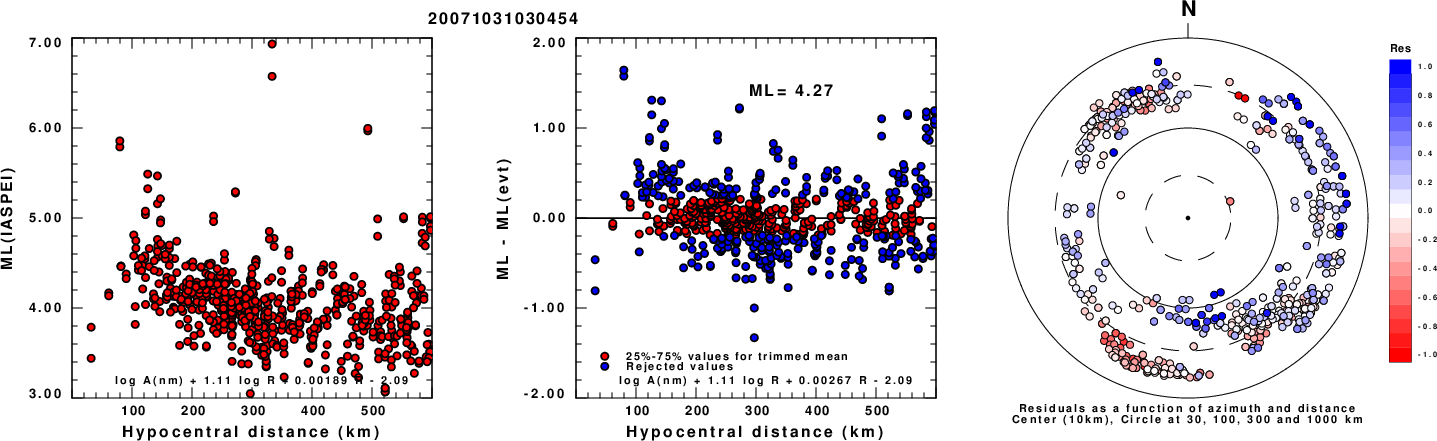
Left: ML computed using the IASPEI formula for Horizontal components. Center: ML residuals computed using a modified IASPEI formula that accounts for path specific attenuation; the values used for the trimmed mean are indicated. The ML relation used for each figure is given at the bottom of each plot.
Right: Residuals from new relation as a function of distance and azimuth.
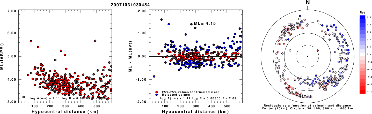
Left: ML computed using the IASPEI formula for Vertical components (research). Center: ML residuals computed using a modified IASPEI formula that accounts for path specific attenuation; the values used for the trimmed mean are indicated. The ML relation used for each figure is given at the bottom of each plot.
Right: Residuals from new relation as a function of distance and azimuth.
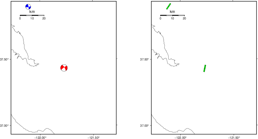
Context
The left panel of the next figure presents the focal mechanism for this earthquake (red) in the context of other nearby events (blue) in the SLU Moment Tensor Catalog. The right panel shows the inferred direction of maximum compressive stress and the type of faulting (green is strike-slip, red is normal, blue is thrust; oblique is shown by a combination of colors). Thus context plot is useful for assessing the appropriateness of the moment tensor of this event.
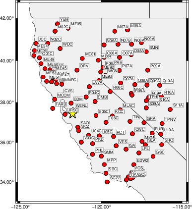
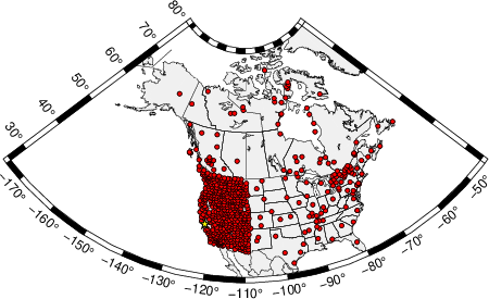
Waveform Inversion using wvfgrd96
The focal mechanism was determined using broadband seismic waveforms. The location of the event (star) and the
stations used for (red) the waveform inversion are shown in the next figure.
|
|
Location of broadband stations used for waveform inversion
|
The program wvfgrd96 was used with good traces observed at short distance to determine the focal mechanism, depth and seismic moment. This technique requires a high quality signal and well determined velocity model for the Green's functions. To the extent that these are the quality data, this type of mechanism should be preferred over the radiation pattern technique which requires the separate step of defining the pressure and tension quadrants and the correct strike.
The observed and predicted traces are filtered using the following gsac commands:
cut o DIST/3.3 -40 o DIST/3.3 +50
rtr
taper w 0.1
hp c 0.03 n 3
lp c 0.06 n 3
The results of this grid search are as follow:
           DEPTH  STK   DIP  RAKE   MW    FIT
WVFGRD96    1.0   235    65    15   5.09 0.1996
WVFGRD96    2.0    60    75    40   5.23 0.2628
WVFGRD96    3.0   235    60    10   5.24 0.2935
WVFGRD96    4.0   230    80   -15   5.26 0.3183
WVFGRD96    5.0   230    75   -15   5.29 0.3400
WVFGRD96    6.0   235    80   -15   5.30 0.3594
WVFGRD96    7.0   235    80   -15   5.33 0.3794
WVFGRD96    8.0   235    80   -20   5.36 0.3976
WVFGRD96    9.0   235    80   -20   5.38 0.4122
WVFGRD96   10.0   235    80   -20   5.40 0.4237
WVFGRD96   11.0   235    80   -20   5.41 0.4331
WVFGRD96   12.0   235    80   -20   5.42 0.4401
WVFGRD96   13.0   235    80   -20   5.44 0.4449
WVFGRD96   14.0   235    80   -20   5.45 0.4476
WVFGRD96   15.0   235    80   -15   5.46 0.4493
WVFGRD96   16.0   235    80   -15   5.47 0.4494
WVFGRD96   17.0   235    80   -15   5.48 0.4486
WVFGRD96   18.0   235    80   -15   5.49 0.4466
WVFGRD96   19.0   235    80   -15   5.50 0.4438
WVFGRD96   20.0   235    80   -15   5.51 0.4396
WVFGRD96   21.0   235    80   -20   5.52 0.4348
WVFGRD96   22.0   235    80   -20   5.53 0.4290
WVFGRD96   23.0   235    80   -20   5.53 0.4223
WVFGRD96   24.0   235    80   -20   5.54 0.4150
WVFGRD96   25.0   235    80   -20   5.55 0.4072
WVFGRD96   26.0   235    75   -15   5.55 0.3992
WVFGRD96   27.0   235    75   -15   5.56 0.3911
WVFGRD96   28.0   235    75   -15   5.57 0.3828
WVFGRD96   29.0   235    75   -15   5.57 0.3742
The best solution is
WVFGRD96 16.0 235 80 -15 5.47 0.4494
The mechanism corresponding to the best fit is
|
|
Figure 1. Waveform inversion focal mechanism
|
The best fit as a function of depth is given in the following figure:
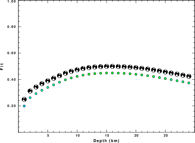
|
|
Figure 2. Depth sensitivity for waveform mechanism
|
The comparison of the observed and predicted waveforms is given in the next figure. The red traces are the observed and the blue are the predicted.
Each observed-predicted component is plotted to the same scale and peak amplitudes are indicated by the numbers to the left of each trace. A pair of numbers is given in black at the right of each predicted traces. The upper number it the time shift required for maximum correlation between the observed and predicted traces. This time shift is required because the synthetics are not computed at exactly the same distance as the observed, the velocity model used in the predictions may not be perfect and the epicentral parameters may be be off.
A positive time shift indicates that the prediction is too fast and should be delayed to match the observed trace (shift to the right in this figure). A negative value indicates that the prediction is too slow. The lower number gives the percentage of variance reduction to characterize the individual goodness of fit (100% indicates a perfect fit).
The bandpass filter used in the processing and for the display was
cut o DIST/3.3 -40 o DIST/3.3 +50
rtr
taper w 0.1
hp c 0.03 n 3
lp c 0.06 n 3

|
|
Figure 3. Waveform comparison for selected depth. Red: observed; Blue - predicted. The time shift with respect to the model prediction is indicated. The percent of fit is also indicated. The time scale is relative to the first trace sample.
|
|
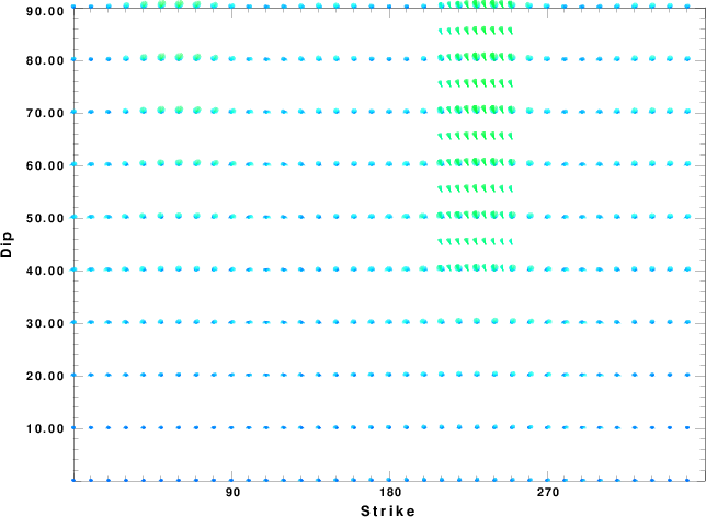
|
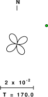
Focal mechanism sensitivity at the preferred depth. The red color indicates a very good fit to the waveforms.
Each solution is plotted as a vector at a given value of strike and dip with the angle of the vector representing the rake angle, measured, with respect to the upward vertical (N) in the figure.
|
A check on the assumed source location is possible by looking at the time shifts between the observed and predicted traces. The time shifts for waveform matching arise for several reasons:
- The origin time and epicentral distance are incorrect
- The velocity model used for the inversion is incorrect
- The velocity model used to define the P-arrival time is not the
same as the velocity model used for the waveform inversion
(assuming that the initial trace alignment is based on the
P arrival time)
Assuming only a mislocation, the time shifts are fit to a functional form:
Time_shift = A + B cos Azimuth + C Sin Azimuth
The time shifts for this inversion lead to the next figure:
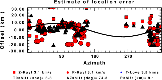
The derived shift in origin time and epicentral coordinates are given at the bottom of the figure.
Surface-Wave Focal Mechanism
The following figure shows the stations used in the grid search for the best focal mechanism to fit the surface-wave spectral amplitudes of the Love and Rayleigh waves.
|
|
Location of broadband stations used to obtain focal mechanism from surface-wave spectral amplitudes
|
The surface-wave determined focal mechanism is shown here.
  NODAL PLANES


  STK=      59.99
  DIP=      80.00
 RAKE=      29.99

             OR

  STK=     324.26
  DIP=      60.51
 RAKE=     168.49


DEPTH = 11.0 km

Mw = 5.54
Best Fit 0.8679 - P-T axis plot gives solutions with FIT greater than FIT90
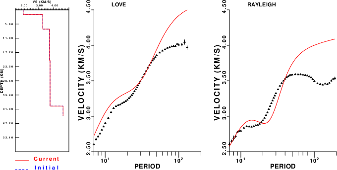
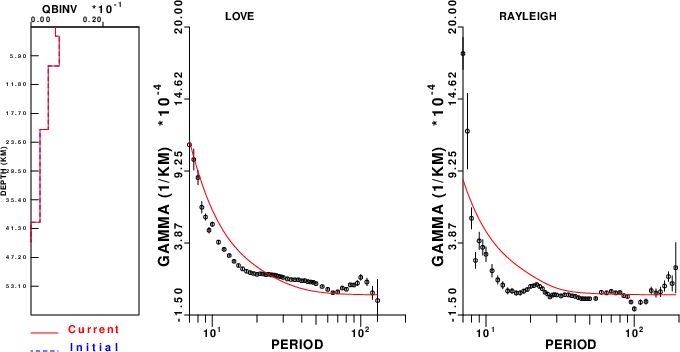
Surface-wave analysis
Surface wave analysis was performed using codes from
Computer Programs in Seismology, specifically the
multiple filter analysis program do_mft and the surface-wave
radiation pattern search program srfgrd96.
Data preparation
Digital data were collected, instrument response removed and traces converted
to Z, R an T components. Multiple filter analysis was applied to the Z and T traces to obtain the Rayleigh- and Love-wave spectral amplitudes, respectively.
These were input to the search program which examined all depths between 1 and 25 km
and all possible mechanisms.
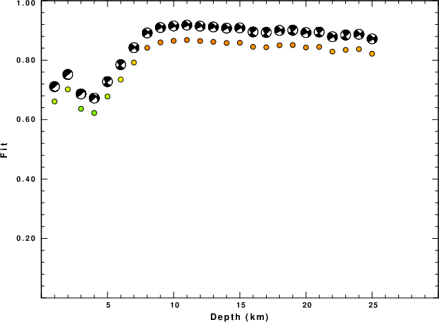
|
|
Best mechanism fit as a function of depth. The preferred depth is given above. Lower hemisphere projection
|
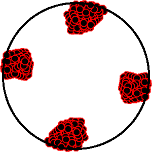
|
|
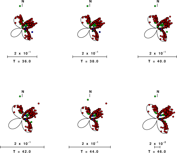
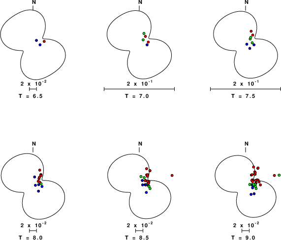
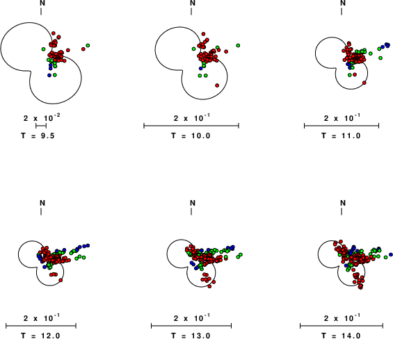
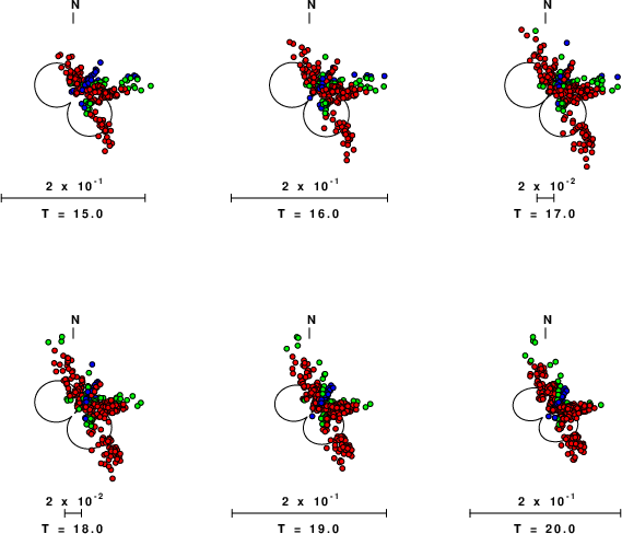
Pressure-tension axis trends. Since the surface-wave spectra search does not distinguish between P and T axes and since there is a 180 ambiguity in strike, all possible P and T axes are plotted. First motion data and waveforms will be used to select the preferred mechanism. The purpose of this plot is to provide an idea of the
possible range of solutions. The P and T-axes for all mechanisms with goodness of fit greater than 0.9 FITMAX (above) are plotted here.
|
|
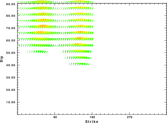
|
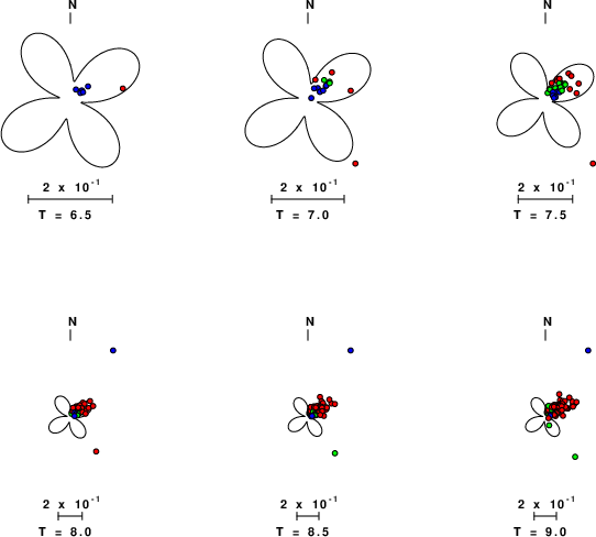
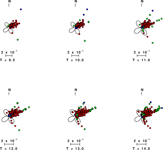
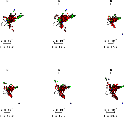
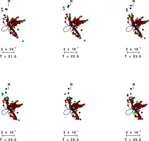
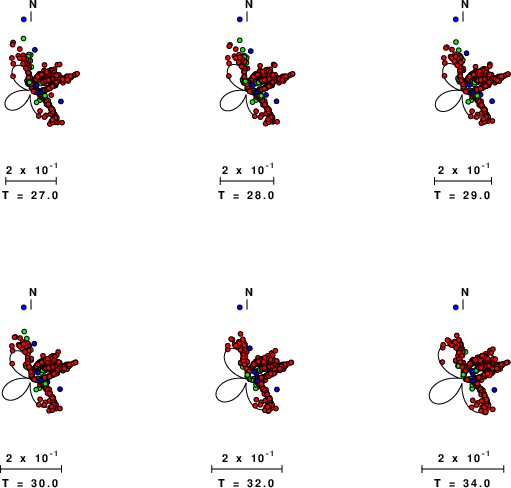
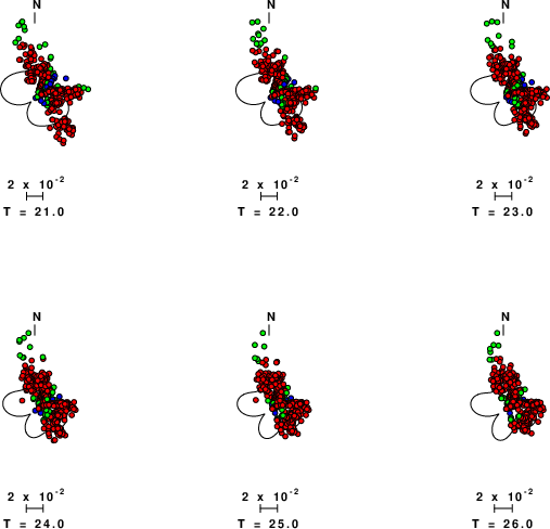
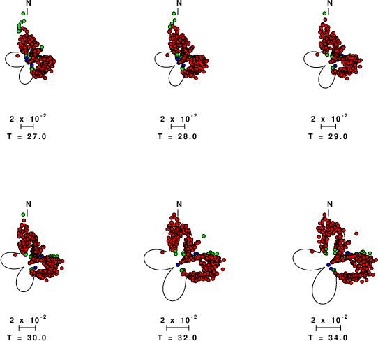
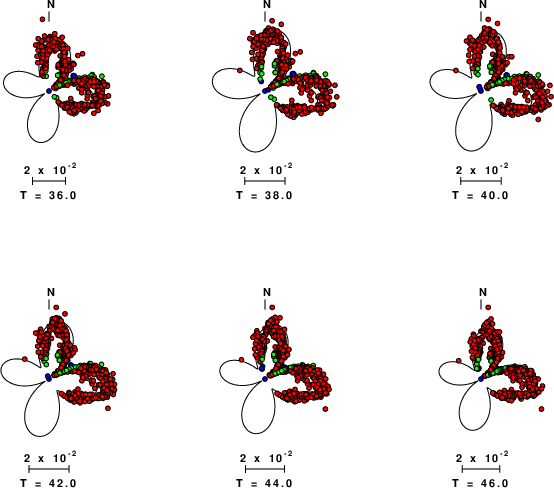
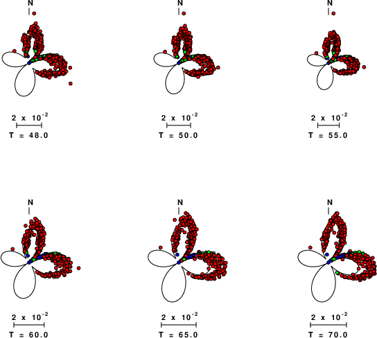
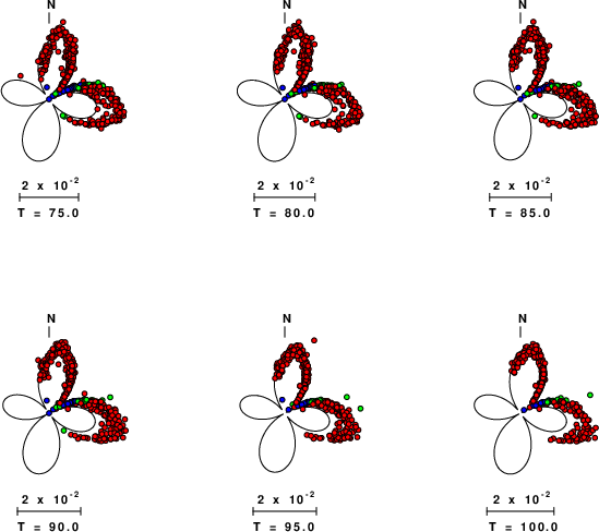
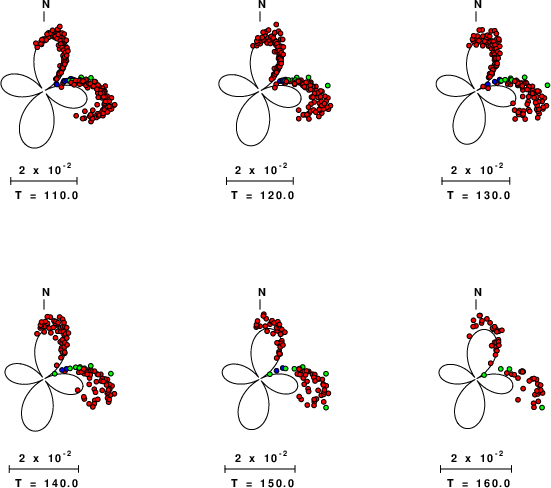
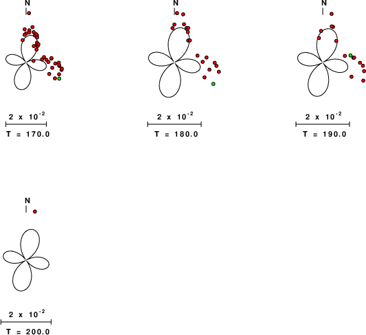
Focal mechanism sensitivity at the preferred depth. The red color indicates a very good fit to the Love and Rayleigh wave radiation patterns.
Each solution is plotted as a vector at a given value of strike and dip with the angle of the vector representing the rake angle, measured, with respect to the upward vertical (N) in the figure. Because of the symmetry of the spectral amplitude rediation patterns, only strikes from 0-180 degrees are sampled.
|
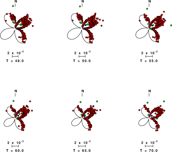
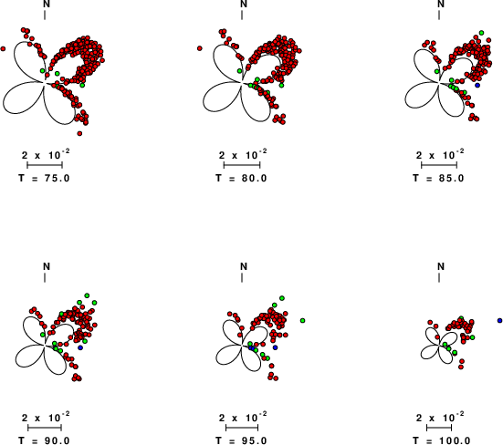
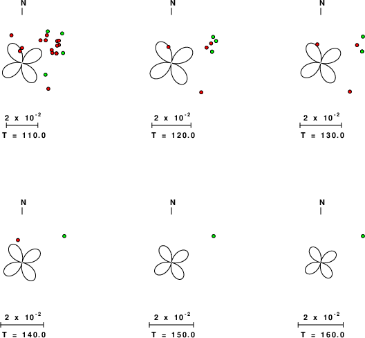
Love-wave radiation patterns
Rayleigh-wave radiation patterns