Location
2010/10/13 14:06:30 35.2020 -97.3090 5.0 4.30 Oklahoma
Arrival Times (from USGS)
Arrival time list
Felt Map
USGS Felt map for this earthquake
USGS Felt reports main page
Focal Mechanism
 USGS/SLU Moment Tensor Solution
 ENS  2010/10/13 14:06:29:0  35.20  -97.31   5.0 4.3 Oklahoma

 Stations used:
   AG.WLAR NM.MGMO NM.UALR TA.129A TA.131A TA.133A TA.134A
   TA.135A TA.137A TA.139A TA.230A TA.231A TA.232A TA.233A
   TA.234A TA.236A TA.332A TA.333A TA.334A TA.335A TA.434A
   TA.435B TA.436A TA.P33A TA.P34A TA.P35A TA.Q30A TA.Q31A
   TA.Q32A TA.Q33A TA.Q34A TA.Q35A TA.Q36A TA.Q37A TA.R29A
   TA.R30A TA.R31A TA.R33A TA.R35A TA.R36A TA.S28A TA.S29A
   TA.S30A TA.S31A TA.S32A TA.S34A TA.S35A TA.S36A TA.T29A
   TA.T30A TA.T31A TA.T32A TA.T33A TA.T34A TA.T35A TA.T36A
   TA.T37A TA.TUL1 TA.U29A TA.U30A TA.U31A TA.U32A TA.U33A
   TA.U34A TA.V29A TA.V32A TA.V33A TA.V34A TA.V35A TA.W31A
   TA.W32A TA.W33A TA.W34A TA.W35A TA.W36A TA.W37A TA.W38A
   TA.WHTX TA.X32A TA.X33A TA.X34A TA.X35A TA.X36A TA.X37A
   TA.X38A TA.Y33A TA.Y34A TA.Y35A TA.Y36A TA.Y37A TA.Y38A
   TA.Y39A TA.Z29A TA.Z31A TA.Z32A TA.Z33A TA.Z34A TA.Z36A
   TA.Z39A US.CBKS US.KSU1 US.MIAR US.WMOK

 Filtering commands used:
   hp c 0.02 n 3
   lp c 0.06 n 3

 Best Fitting Double Couple
  Mo = 3.94e+22 dyne-cm
  Mw = 4.33
  Z  = 14 km
  Plane   Strike  Dip  Rake
   NP1       29    85   170
   NP2      120    80     5
  Principal Axes:
   Axis    Value   Plunge  Azimuth
    T   3.94e+22     11     344
    N   0.00e+00     79     183
    P  -3.94e+22      4      75

 Moment Tensor: (dyne-cm)
    Component   Value
       Mxx     3.26e+22
       Mxy    -1.98e+22
       Mxz     6.20e+21
       Myy    -3.37e+22
       Myz    -4.28e+21
       Mzz     1.17e+21


                        ###########
                 #### T ##############-
              #######   #############-----
             #######################-------
           #########################---------
          #########################-----------
         ---######################-------------
        ------###################-------------
        --------################-------------- P
       ------------############---------------
       ---------------########-------------------
       ------------------####--------------------
       ------------------------------------------
        -------------------####-----------------
        ------------------#########-------------
         ----------------##############--------
          -------------######################-
           -----------#######################
             --------######################
              ------######################
                 -#####################
                     ##############


 Global CMT Convention Moment Tensor:
      R          T          P
  1.17e+21   6.20e+21   4.28e+21
  6.20e+21   3.26e+22   1.98e+22
  4.28e+21   1.98e+22  -3.37e+22


Details of the solution is found at

http://www.eas.slu.edu/eqc/eqc_mt/MECH.NA/20101013140629/index.html
|
Preferred Solution
The preferred solution from an analysis of the surface-wave spectral amplitude radiation pattern, waveform inversion and first motion observations is
      STK = 120
      DIP = 80
     RAKE = 5
       MW = 4.33
       HS = 14.0
The waveform inversion is preferred.
Moment Tensor Comparison
The following compares this source inversion to others
| SLU |
GCMT |
SLUFM |
 USGS/SLU Moment Tensor Solution
 ENS  2010/10/13 14:06:29:0  35.20  -97.31   5.0 4.3 Oklahoma

 Stations used:
   AG.WLAR NM.MGMO NM.UALR TA.129A TA.131A TA.133A TA.134A
   TA.135A TA.137A TA.139A TA.230A TA.231A TA.232A TA.233A
   TA.234A TA.236A TA.332A TA.333A TA.334A TA.335A TA.434A
   TA.435B TA.436A TA.P33A TA.P34A TA.P35A TA.Q30A TA.Q31A
   TA.Q32A TA.Q33A TA.Q34A TA.Q35A TA.Q36A TA.Q37A TA.R29A
   TA.R30A TA.R31A TA.R33A TA.R35A TA.R36A TA.S28A TA.S29A
   TA.S30A TA.S31A TA.S32A TA.S34A TA.S35A TA.S36A TA.T29A
   TA.T30A TA.T31A TA.T32A TA.T33A TA.T34A TA.T35A TA.T36A
   TA.T37A TA.TUL1 TA.U29A TA.U30A TA.U31A TA.U32A TA.U33A
   TA.U34A TA.V29A TA.V32A TA.V33A TA.V34A TA.V35A TA.W31A
   TA.W32A TA.W33A TA.W34A TA.W35A TA.W36A TA.W37A TA.W38A
   TA.WHTX TA.X32A TA.X33A TA.X34A TA.X35A TA.X36A TA.X37A
   TA.X38A TA.Y33A TA.Y34A TA.Y35A TA.Y36A TA.Y37A TA.Y38A
   TA.Y39A TA.Z29A TA.Z31A TA.Z32A TA.Z33A TA.Z34A TA.Z36A
   TA.Z39A US.CBKS US.KSU1 US.MIAR US.WMOK

 Filtering commands used:
   hp c 0.02 n 3
   lp c 0.06 n 3

 Best Fitting Double Couple
  Mo = 3.94e+22 dyne-cm
  Mw = 4.33
  Z  = 14 km
  Plane   Strike  Dip  Rake
   NP1       29    85   170
   NP2      120    80     5
  Principal Axes:
   Axis    Value   Plunge  Azimuth
    T   3.94e+22     11     344
    N   0.00e+00     79     183
    P  -3.94e+22      4      75

 Moment Tensor: (dyne-cm)
    Component   Value
       Mxx     3.26e+22
       Mxy    -1.98e+22
       Mxz     6.20e+21
       Myy    -3.37e+22
       Myz    -4.28e+21
       Mzz     1.17e+21


                        ###########
                 #### T ##############-
              #######   #############-----
             #######################-------
           #########################---------
          #########################-----------
         ---######################-------------
        ------###################-------------
        --------################-------------- P
       ------------############---------------
       ---------------########-------------------
       ------------------####--------------------
       ------------------------------------------
        -------------------####-----------------
        ------------------#########-------------
         ----------------##############--------
          -------------######################-
           -----------#######################
             --------######################
              ------######################
                 -#####################
                     ##############


 Global CMT Convention Moment Tensor:
      R          T          P
  1.17e+21   6.20e+21   4.28e+21
  6.20e+21   3.26e+22   1.98e+22
  4.28e+21   1.98e+22  -3.37e+22


Details of the solution is found at

http://www.eas.slu.edu/eqc/eqc_mt/MECH.NA/20101013140629/index.html
|
October 13, 2010, OKLAHOMA, MW=4.4

Meredith Nettles
Goran Ekstrom

CENTROID-MOMENT-TENSOR  SOLUTION
GCMT EVENT:     S201010131406A
DATA: TA US IU II CU G
SURFACE WAVES: 285S, 377C, T= 40
TIMESTAMP:      Q-20101014143127
CENTROID LOCATION:
ORIGIN TIME:      14:06:31.7 0.2
LAT:35.21N 0.01;LON: 97.28W 0.02
DEP: 12.0  FIX;TRIANG HDUR:  1.0
MOMENT TENSOR: SCALE 10**22 D-CM
RR=-0.032 0.139; TT= 3.830 0.108
PP=-3.800 0.144; RT= 0.847 0.313
RP=-0.261 0.365; TP= 2.310 0.119
PRINCIPAL AXES:
1.(T) VAL=  4.596;PLG= 9;AZM=345
2.(N)      -0.100;    79;    130
3.(P)      -4.497;     6;    254
BEST DBLE.COUPLE:M0= 4.55*10**22
NP1: STRIKE= 29;DIP=79;SLIP= 178
NP2: STRIKE=120;DIP=88;SLIP=  11

               ########
        #### T ##########--
      ######   ##########----
    ####################-------
   #####################--------
  ----#################----------
  -------#############-----------
 -----------#########-------------
 --------------######-------------
 -----------------##--------------
    --------------####------------
  P -------------########--------
    ------------############-----
   ------------#################
    ----------#################
      ------#################
        --#################
            ###########
|

First motions and takeoff angles from an elocate run.
|
Waveform Inversion
The focal mechanism was determined using broadband seismic waveforms. The location of the event and the
and stations used for the waveform inversion are shown in the next figure.

|
|
Location of broadband stations used for waveform inversion
|
The program wvfgrd96 was used with good traces observed at short distance to determine the focal mechanism, depth and seismic moment. This technique requires a high quality signal and well determined velocity model for the Green functions. To the extent that these are the quality data, this type of mechanism should be preferred over the radiation pattern technique which requires the separate step of defining the pressure and tension quadrants and the correct strike.
The observed and predicted traces are filtered using the following gsac commands:
hp c 0.02 n 3
lp c 0.06 n 3
The results of this grid search from 0.5 to 19 km depth are as follow:
           DEPTH  STK   DIP  RAKE   MW    FIT
WVFGRD96    0.5   120    65     0   4.17 0.4012
WVFGRD96    1.0   120    65     0   4.19 0.4196
WVFGRD96    2.0   120    70     0   4.21 0.4487
WVFGRD96    3.0   120    70     0   4.23 0.4688
WVFGRD96    4.0   120    70     0   4.25 0.4843
WVFGRD96    5.0   120    70     5   4.26 0.4973
WVFGRD96    6.0   120    75    10   4.27 0.5092
WVFGRD96    7.0   120    75    10   4.28 0.5198
WVFGRD96    8.0   120    75    10   4.29 0.5285
WVFGRD96    9.0   120    75     5   4.30 0.5356
WVFGRD96   10.0   120    75    10   4.31 0.5422
WVFGRD96   11.0   120    75     5   4.31 0.5461
WVFGRD96   12.0   120    75     5   4.32 0.5487
WVFGRD96   13.0   120    75     5   4.33 0.5498
WVFGRD96   14.0   120    80     5   4.33 0.5506
WVFGRD96   15.0   120    80     5   4.34 0.5501
WVFGRD96   16.0   120    80     5   4.35 0.5489
WVFGRD96   17.0   120    80     5   4.36 0.5472
WVFGRD96   18.0   120    80     5   4.36 0.5447
WVFGRD96   19.0   120    80     5   4.37 0.5419
WVFGRD96   20.0   120    80     5   4.38 0.5387
WVFGRD96   21.0   120    80     5   4.39 0.5339
WVFGRD96   22.0   120    80     5   4.39 0.5288
WVFGRD96   23.0   120    80     5   4.40 0.5230
WVFGRD96   24.0   120    80     5   4.40 0.5167
WVFGRD96   25.0   120    80     5   4.41 0.5102
WVFGRD96   26.0   120    80     5   4.41 0.5032
WVFGRD96   27.0   120    80     5   4.42 0.4959
WVFGRD96   28.0   120    80     5   4.42 0.4885
WVFGRD96   29.0   120    80     5   4.43 0.4810
The best solution is
WVFGRD96 14.0 120 80 5 4.33 0.5506
The mechanism correspond to the best fit is

|
|
Figure 1. Waveform inversion focal mechanism
|
The best fit as a function of depth is given in the following figure:

|
|
Figure 2. Depth sensitivity for waveform mechanism
|
The comparison of the observed and predicted waveforms is given in the next figure. The red traces are the observed and the blue are the predicted.
Each observed-predicted component is plotted to the same scale and peak amplitudes are indicated by the numbers to the left of each trace. A pair of numbers is given in black at the right of each predicted traces. The upper number it the time shift required for maximum correlation between the observed and predicted traces. This time shift is required because the synthetics are not computed at exactly the same distance as the observed and because the velocity model used in the predictions may not be perfect.
A positive time shift indicates that the prediction is too fast and should be delayed to match the observed trace (shift to the right in this figure). A negative value indicates that the prediction is too slow. The lower number gives the percentage of variance reduction to characterize the individual goodness of fit (100% indicates a perfect fit).
The bandpass filter used in the processing and for the display was
hp c 0.02 n 3
lp c 0.06 n 3

|
|
Figure 3. Waveform comparison for selected depth
|

|
|
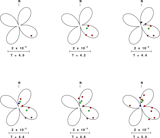
Focal mechanism sensitivity at the preferred depth. The red color indicates a very good fit to thewavefroms.
Each solution is plotted as a vector at a given value of strike and dip with the angle of the vector representing the rake angle, measured, with respect to the upward vertical (N) in the figure.
|
A check on the assumed source location is possible by looking at the time shifts between the observed and predicted traces. The time shifts for waveform matching arise for several reasons:
- The origin time and epicentral distance are incorrect
- The velocity model used for the inversion is incorrect
- The velocity model used to define the P-arrival time is not the
same as the velocity model used for the waveform inversion
(assuming that the initial trace alignment is based on the
P arrival time)
Assuming only a mislocation, the time shifts are fit to a functional form:
Time_shift = A + B cos Azimuth + C Sin Azimuth
The time shifts for this inversion lead to the next figure:

The derived shift in origin time and epicentral coordinates are given at the bottom of the figure.
Surface-Wave Focal Mechanism
The following figure shows the stations used in the grid search for the best focal mechanism to fit the surface-wave spectral amplitudes of the Love and Rayleigh waves.

|
|
Location of broadband stations used to obtain focal mechanism from surface-wave spectral amplitudes
|
The surface-wave determined focal mechanism is shown here.
  NODAL PLANES


  STK=      27.38
  DIP=      80.34
 RAKE=     164.78

             OR

  STK=     119.99
  DIP=      75.00
 RAKE=      10.00


DEPTH = 11.0 km

Mw = 4.37
Best Fit 0.8852 - P-T axis plot gives solutions with FIT greater than FIT90
First motion data
The P-wave first motion data for focal mechanism studies are as follow:
Sta Az Dist First motion
Surface-wave analysis
Surface wave analysis was performed using codes from
Computer Programs in Seismology, specifically the
multiple filter analysis program do_mft and the surface-wave
radiation pattern search program srfgrd96.
Data preparation
Digital data were collected, instrument response removed and traces converted
to Z, R an T components. Multiple filter analysis was applied to the Z and T traces to obtain the Rayleigh- and Love-wave spectral amplitudes, respectively.
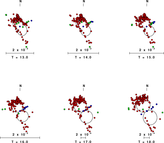
These were input to the search program which examined all depths between 1 and 25 km
and all possible mechanisms.

|
|
Best mechanism fit as a function of depth. The preferred depth is given above. Lower hemisphere projection
|

|
|
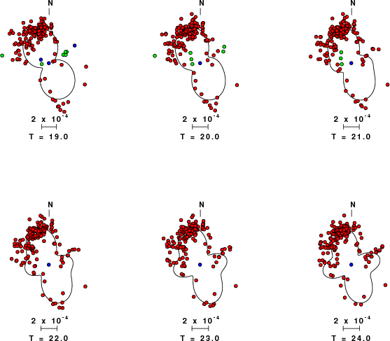
Pressure-tension axis trends. Since the surface-wave spectra search does not distinguish between P and T axes and since there is a 180 ambiguity in strike, all possible P and T axes are plotted. First motion data and waveforms will be used to select the preferred mechanism. The purpose of this plot is to provide an idea of the
possible range of solutions. The P and T-axes for all mechanisms with goodness of fit greater than 0.9 FITMAX (above) are plotted here.
|

|
|
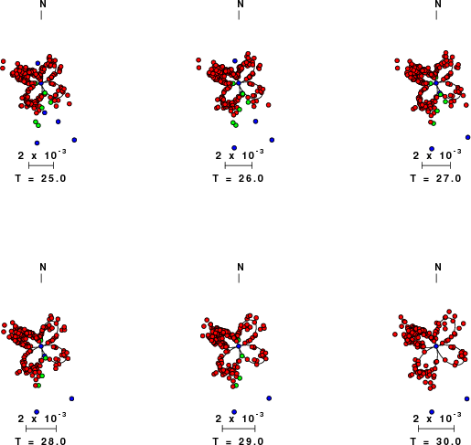
Focal mechanism sensitivity at the preferred depth. The red color indicates a very good fit to the Love and Rayleigh wave radiation patterns.
Each solution is plotted as a vector at a given value of strike and dip with the angle of the vector representing the rake angle, measured, with respect to the upward vertical (N) in the figure. Because of the symmetry of the spectral amplitude rediation patterns, only strikes from 0-180 degrees are sampled.
|
Love-wave radiation patterns
Rayleigh-wave radiation patterns
Broadband station distribution
The distribution of broadband stations with azimuth and distance is
Listing of broadband stations used
Waveform comparison for this mechanism
Since the analysis of the surface-wave radiation patterns uses only spectral
amplitudes and because the surfave-wave radiation patterns have a 180 degree symmetry, each surface-wave solution consists of four possible focal mechanisms corresponding to the interchange of the P- and T-axes and a roation of the mechanism by 180 degrees. To select one mechanism, P-wave first motion can be used. This was not possible in this case because all the P-wave first motions were
emergent ( a feature of the P-wave wave takeoff angle, the station location and the mechanism). The other way to select among the mechanisms is to compute
forward synthetics and compare the observed and predicted waveforms.
The fits to the waveforms with the given mechanism are show below:
This figure shows the fit to the three components of motion (Z - vertical, R-radial and T - transverse). For each station and component, the
observed traces is shown in red and the model predicted trace in blue. The traces represent filtered ground velocity in units of meters/sec (the peak value is printed adjacent to each trace; each pair of traces to plotted to the same scale to emphasize the difference in levels). Both synthetic and observed traces have been filtered using the SAC commands:
Discussion
The Future
Should the national backbone of the
USGS Advanced National Seismic System (ANSS)
be implemented with an interstation separation of 300 km, it is very likely that
an earthquake such as this would have been recorded at distances on the order of
100-200 km. This means that the closest station would have information on
source depth and mechanism that was lacking here.
Acknowledgements
Dr. Harley Benz, USGS, provided the USGS USNSN digital data.
The digital data used in this study were provided by Natural Resources Canada through their AUTODRM site http://www.seismo.nrcan.gc.ca/nwfa/autodrm/autodrm_req_e.php, and IRIS using their BUD interface.
Thanks also to the many seismic network operators whose dedication make this effort possible: University of Alaska, University of Washington, Oregon State University, University of Utah, Montana Bureas of Mines, UC Berkely, Caltech, UC San Diego, Saint L ouis University, Universityof Memphis, Lamont Doehrty Earth Observatory, Boston College, the Iris stations and the Transportable Array of EarthScope.
Appendix A
Spectra fit plots to each station
NetQuake Recordings
Local Netquake recorders recorded this earthquake. They were at distances of 35 - 50 km from the epicenter. The presentation is given at the link netquake.html
Velocity Model
The CUS used for the waveform synthetic seismograms and for the surface wave eigenfunctions and dispersion is as follows:
MODEL.01
CUS Model with Q from simple gamma values
ISOTROPIC
KGS
FLAT EARTH
1-D
CONSTANT VELOCITY
LINE08
LINE09
LINE10
LINE11
  H(KM) VP(KM/S) VS(KM/S) RHO(GM/CC)   QP   QS  ETAP  ETAS  FREFP  FREFS
  1.0000  5.0000  2.8900  2.5000 0.172E-02 0.387E-02 0.00  0.00  1.00  1.00
  9.0000  6.1000  3.5200  2.7300 0.160E-02 0.363E-02 0.00  0.00  1.00  1.00
 10.0000  6.4000  3.7000  2.8200 0.149E-02 0.336E-02 0.00  0.00  1.00  1.00
 20.0000  6.7000  3.8700  2.9020 0.000E-04 0.000E-04 0.00  0.00  1.00  1.00
  0.0000  8.1500  4.7000  3.3640 0.194E-02 0.431E-02 0.00  0.00  1.00  1.00
Quality Control
Here we tabulate the reasons for not using certain digital data sets
The following stations did not have a valid response files:
DATE=Fri Oct 15 16:54:41 CDT 2010
Last Changed 2010/10/13


