
The Geological Survey of Canada (Natural Resources Canada) solution is preferred.
The initial source inversion was obtained using the NEIC solution. The goodness of fit was quite good, but there were very large time shifts required to fit the waveforms. Such time shifts are indicative of the use of an incorrect velocity model, or a poor location. To examine this the time shifts can be decomposed into a common offset and an azimuthal component. For this event, the time shifts on the vertical and radial compoents were converted to a kilometer difference in epicentral distance by assuming a constant group velocity of 3.1 km/s for the Rayleigh wave pulse; a group velocity of 3.5 km/s was assumed for the Love wave pulse on the transverse component. An obvious azimuthal effect was observed, as shown in the next figure.
A positive time shift in the comparison of observed and predicted waveforms, as seen below, means that the predicted trace must be moved later in time which would occur if the actual velocity model is slower than assumed, if the origin time is actually later, or if the epicentral distance is greater than assumed. The previous figure assumes that the shift is due to a mislocation. Thus a positive time shift means that the assumed epicentral distance is too small, ro that the epicenter must be moved away from the station.
The NRCAN solution leads to the tiem shifts seen below. The delay plot is givne in the next figure.

It is obvious that the spatial shifts are smaller than for the NEIC solution.
This technique is similar to that used for telseismic earqhauke location. The only real problem is that the actual pulse being matched by the time shift is dispersed, and the assumption of a single group velocity is not correct.
2010/09/04 00:23:11.35 62.864 -125.821 1.0 4.8 ML 120 km of Wrigley, NT
2010/09/04 00:23:13 62.943 -125.718 7.1 4.50 NT, Canada
USGS Felt map for this earthquake
 USGS/SLU Moment Tensor Solution
 ENS  2010/09/04 00:23:11:3  62.86 -125.82   1.0 4.8 NT, Canada

 Stations used:
   AK.BAL AK.BESE AK.CTG AK.DCPH AK.PIN AT.SKAG AT.YKU2
   CN.CLVN CN.COKN CN.DHRN CN.DLBC CN.HPLN CN.HYT CN.INK
   CN.KUKN CN.SMPN CN.WHY CN.YKW3 CN.YUK5 US.EGAK US.WRAK

 Filtering commands used:
   hp c 0.02 n 3
   lp c 0.10 n 3

 Best Fitting Double Couple
  Mo = 9.89e+21 dyne-cm
  Mw = 3.93
  Z  = 11 km
  Plane   Strike  Dip  Rake
   NP1      310    85   -60
   NP2       49    30   -170
  Principal Axes:
   Axis    Value   Plunge  Azimuth
    T   9.89e+21     33      15
    N   0.00e+00     30     127
    P  -9.89e+21     42     248

 Moment Tensor: (dyne-cm)
    Component   Value
       Mxx     5.72e+21
       Mxy    -1.23e+20
       Mxz     6.18e+21
       Myy    -4.23e+21
       Myz     5.75e+21
       Mzz    -1.49e+21


                     ##############
                 ######################
              ################   #########
             ################# T ##########
           ---################   ###########-
          -------############################-
         -----------#########################--
        --------------#######################---
        ----------------#####################---
       --------------------##################----
       ----------------------################----
       ------------------------#############-----
       --------   ---------------###########-----
        ------- P -----------------########-----
        -------   -------------------#####------
         ------------------------------#-------
          ----------------------------###-----
           -------------------------#######--
             ---------------------#########
              ###------------#############
                 ######################
                     ##############


 Global CMT Convention Moment Tensor:
      R          T          P
 -1.49e+21   6.18e+21  -5.75e+21
  6.18e+21   5.72e+21   1.23e+20
 -5.75e+21   1.23e+20  -4.23e+21


Details of the solution is found at

http://www.eas.slu.edu/eqc/eqc_mt/MECH.NA/20100904002311/index.html
|
      STK = 310
      DIP = 85
     RAKE = -60
       MW = 3.93
       HS = 11.0
The waveform inversion is preferred. However the surface-wave spectral amplitude technique was applied because of the lack of good azimuthal coverThe moment magnitudes are similar as is the mechanism, The depths disagree.
The following compares this source inversion to others
 USGS/SLU Moment Tensor Solution
 ENS  2010/09/04 00:23:11:3  62.86 -125.82   1.0 4.8 NT, Canada

 Stations used:
   AK.BAL AK.BESE AK.CTG AK.DCPH AK.PIN AT.SKAG AT.YKU2
   CN.CLVN CN.COKN CN.DHRN CN.DLBC CN.HPLN CN.HYT CN.INK
   CN.KUKN CN.SMPN CN.WHY CN.YKW3 CN.YUK5 US.EGAK US.WRAK

 Filtering commands used:
   hp c 0.02 n 3
   lp c 0.10 n 3

 Best Fitting Double Couple
  Mo = 9.89e+21 dyne-cm
  Mw = 3.93
  Z  = 11 km
  Plane   Strike  Dip  Rake
   NP1      310    85   -60
   NP2       49    30   -170
  Principal Axes:
   Axis    Value   Plunge  Azimuth
    T   9.89e+21     33      15
    N   0.00e+00     30     127
    P  -9.89e+21     42     248

 Moment Tensor: (dyne-cm)
    Component   Value
       Mxx     5.72e+21
       Mxy    -1.23e+20
       Mxz     6.18e+21
       Myy    -4.23e+21
       Myz     5.75e+21
       Mzz    -1.49e+21


                     ##############
                 ######################
              ################   #########
             ################# T ##########
           ---################   ###########-
          -------############################-
         -----------#########################--
        --------------#######################---
        ----------------#####################---
       --------------------##################----
       ----------------------################----
       ------------------------#############-----
       --------   ---------------###########-----
        ------- P -----------------########-----
        -------   -------------------#####------
         ------------------------------#-------
          ----------------------------###-----
           -------------------------#######--
             ---------------------#########
              ###------------#############
                 ######################
                     ##############


 Global CMT Convention Moment Tensor:
      R          T          P
 -1.49e+21   6.18e+21  -5.75e+21
  6.18e+21   5.72e+21   1.23e+20
 -5.75e+21   1.23e+20  -4.23e+21


Details of the solution is found at

http://www.eas.slu.edu/eqc/eqc_mt/MECH.NA/20100904002311/index.html
|
The focal mechanism was determined using broadband seismic waveforms. The location of the event and the and stations used for the waveform inversion are shown in the next figure.

|
|
|
The program wvfgrd96 was used with good traces observed at short distance to determine the focal mechanism, depth and seismic moment. This technique requires a high quality signal and well determined velocity model for the Green functions. To the extent that these are the quality data, this type of mechanism should be preferred over the radiation pattern technique which requires the separate step of defining the pressure and tension quadrants and the correct strike.
The observed and predicted traces are filtered using the following gsac commands:
hp c 0.02 n 3
lp c 0.10 n 3
The results of this grid search from 0.5 to 19 km depth are as follow:
           DEPTH  STK   DIP  RAKE   MW    FIT
WVFGRD96    0.5   295    60    65   3.83 0.5055
WVFGRD96    1.0   120    35    65   3.87 0.5164
WVFGRD96    2.0   135    30    90   3.97 0.5095
WVFGRD96    3.0   140    30    95   4.00 0.4664
WVFGRD96    4.0   140    80    65   3.91 0.4740
WVFGRD96    5.0   135    85    65   3.89 0.4986
WVFGRD96    6.0   310    90   -60   3.89 0.5182
WVFGRD96    7.0   135    90    60   3.88 0.5344
WVFGRD96    8.0   135    90    60   3.89 0.5463
WVFGRD96    9.0   135    90    55   3.90 0.5546
WVFGRD96   10.0   310    85   -60   3.93 0.5610
WVFGRD96   11.0   310    85   -60   3.93 0.5638
WVFGRD96   12.0   310    80   -60   3.95 0.5636
WVFGRD96   13.0   310    80   -60   3.95 0.5619
WVFGRD96   14.0   310    80   -60   3.96 0.5576
WVFGRD96   15.0   310    80   -60   3.97 0.5510
WVFGRD96   16.0   310    75   -60   3.99 0.5430
WVFGRD96   17.0   310    75   -60   3.99 0.5338
WVFGRD96   18.0   310    75   -60   4.00 0.5234
WVFGRD96   19.0   310    75   -60   4.01 0.5125
WVFGRD96   20.0   310    75   -60   4.04 0.5011
WVFGRD96   21.0   310    75   -60   4.05 0.4870
WVFGRD96   22.0   310    75   -60   4.06 0.4726
WVFGRD96   23.0   315    70   -60   4.07 0.4579
WVFGRD96   24.0   315    70   -60   4.08 0.4436
WVFGRD96   25.0   310    65   -65   4.08 0.4294
WVFGRD96   26.0   310    65   -65   4.09 0.4150
WVFGRD96   27.0   140    35   -85   4.09 0.4042
WVFGRD96   28.0   140    35   -85   4.10 0.3930
WVFGRD96   29.0   145    35   -80   4.10 0.3816
The best solution is
WVFGRD96 11.0 310 85 -60 3.93 0.5638
The mechanism correspond to the best fit is

|
|
|
The best fit as a function of depth is given in the following figure:

|
|
|
The comparison of the observed and predicted waveforms is given in the next figure. The red traces are the observed and the blue are the predicted. Each observed-predicted componnet is plotted to the same scale and peak amplitudes are indicated by the numbers to the left of each trace. The number in black at the rightr of each predicted traces it the time shift required for maximum correlation between the observed and predicted traces. This time shift is required because the synthetics are not computed at exactly the same distance as the observed and because the velocity model used in the predictions may not be perfect. A positive time shift indicates that the prediction is too fast and should be delayed to match the observed trace (shift to the right in this figure). A negative value indicates that the prediction is too slow. The bandpass filter used in the processing and for the display was
hp c 0.02 n 3
lp c 0.10 n 3

|
|
|

|
| Focal mechanism sensitivity at the preferred depth. The red color indicates a very good fit to thewavefroms. Each solution is plotted as a vector at a given value of strike and dip with the angle of the vector representing the rake angle, measured, with respect to the upward vertical (N) in the figure. |
The following figure shows the stations used in the grid search for the best focal mechanism to fit the surface-wave spectral amplitudes of the Love and Rayleigh waves.

|
|
|
The surface-wave determined focal mechanism is shown here.
  NODAL PLANES


  STK=     326.51
  DIP=      60.50
 RAKE=      95.73

             OR

  STK=     135.00
  DIP=      30.00
 RAKE=      80.00


DEPTH = 6.0 km

Mw = 4.08
Best Fit 0.8033 - P-T axis plot gives solutions with FIT greater than FIT90
 |
The P-wave first motion data for focal mechanism studies are as follow:
Sta Az Dist First motion
Surface wave analysis was performed using codes from Computer Programs in Seismology, specifically the multiple filter analysis program do_mft and the surface-wave radiation pattern search program srfgrd96.
Digital data were collected, instrument response removed and traces converted
to Z, R an T components. Multiple filter analysis was applied to the Z and T traces to obtain the Rayleigh- and Love-wave spectral amplitudes, respectively.
These were input to the search program which examined all depths between 1 and 25 km
and all possible mechanisms.

|
|
|

|
| Pressure-tension axis trends. Since the surface-wave spectra search does not distinguish between P and T axes and since there is a 180 ambiguity in strike, all possible P and T axes are plotted. First motion data and waveforms will be used to select the preferred mechanism. The purpose of this plot is to provide an idea of the possible range of solutions. The P and T-axes for all mechanisms with goodness of fit greater than 0.9 FITMAX (above) are plotted here. |

|
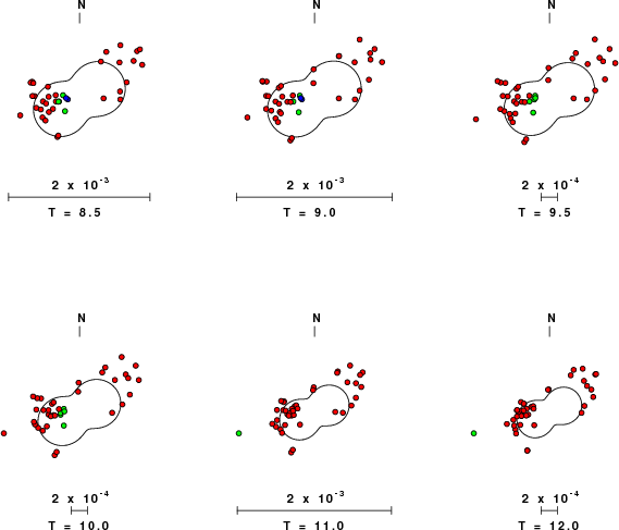
| Focal mechanism sensitivity at the preferred depth. The red color indicates a very good fit to the Love and Rayleigh wave radiation patterns. Each solution is plotted as a vector at a given value of strike and dip with the angle of the vector representing the rake angle, measured, with respect to the upward vertical (N) in the figure. Because of the symmetry of the spectral amplitude rediation patterns, only strikes from 0-180 degrees are sampled. |
The distribution of broadband stations with azimuth and distance is
Listing of broadband stations used
Since the analysis of the surface-wave radiation patterns uses only spectral amplitudes and because the surfave-wave radiation patterns have a 180 degree symmetry, each surface-wave solution consists of four possible focal mechanisms corresponding to the interchange of the P- and T-axes and a roation of the mechanism by 180 degrees. To select one mechanism, P-wave first motion can be used. This was not possible in this case because all the P-wave first motions were emergent ( a feature of the P-wave wave takeoff angle, the station location and the mechanism). The other way to select among the mechanisms is to compute forward synthetics and compare the observed and predicted waveforms.
The fits to the waveforms with the given mechanism are show below:

|
This figure shows the fit to the three components of motion (Z - vertical, R-radial and T - transverse). For each station and component, the observed traces is shown in red and the model predicted trace in blue. The traces represent filtered ground velocity in units of meters/sec (the peak value is printed adjacent to each trace; each pair of traces to plotted to the same scale to emphasize the difference in levels). Both synthetic and observed traces have been filtered using the SAC commands:

|

|
Should the national backbone of the USGS Advanced National Seismic System (ANSS) be implemented with an interstation separation of 300 km, it is very likely that an earthquake such as this would have been recorded at distances on the order of 100-200 km. This means that the closest station would have information on source depth and mechanism that was lacking here.
Dr. Harley Benz, USGS, provided the USGS USNSN digital data. The digital data used in this study were provided by Natural Resources Canada through their AUTODRM site http://www.seismo.nrcan.gc.ca/nwfa/autodrm/autodrm_req_e.php, and IRIS using their BUD interface.
Thanks also to the many seismic network operators whose dedication make this effort possible: University of Alaska, University of Washington, Oregon State University, University of Utah, Montana Bureas of Mines, UC Berkely, Caltech, UC San Diego, Saint L ouis University, Universityof Memphis, Lamont Doehrty Earth Observatory, Boston College, the Iris stations and the Transportable Array of EarthScope.
The CUS used for the waveform synthetic seismograms and for the surface wave eigenfunctions and dispersion is as follows:
MODEL.01
CUS Model with Q from simple gamma values
ISOTROPIC
KGS
FLAT EARTH
1-D
CONSTANT VELOCITY
LINE08
LINE09
LINE10
LINE11
  H(KM) VP(KM/S) VS(KM/S) RHO(GM/CC)   QP   QS  ETAP  ETAS  FREFP  FREFS
  1.0000  5.0000  2.8900  2.5000 0.172E-02 0.387E-02 0.00  0.00  1.00  1.00
  9.0000  6.1000  3.5200  2.7300 0.160E-02 0.363E-02 0.00  0.00  1.00  1.00
 10.0000  6.4000  3.7000  2.8200 0.149E-02 0.336E-02 0.00  0.00  1.00  1.00
 20.0000  6.7000  3.8700  2.9020 0.000E-04 0.000E-04 0.00  0.00  1.00  1.00
  0.0000  8.1500  4.7000  3.3640 0.194E-02 0.431E-02 0.00  0.00  1.00  1.00
Here we tabulate the reasons for not using certain digital data sets
The following stations did not have a valid response files:
DATE=Sat Sep 4 20:32:38 CDT 2010