
2010/06/23 17:41:42 45.904 -75.497 16.4 5.00 Quebec - NRCAN
2010/06/23 17:41:42 45.862 -75.457 18.0 5.00 Quebec - USGS
USGS Felt map for this earthquake
 USGS/SLU Moment Tensor Solution
 ENS  2010/06/23 17:41:42:0  45.86  -75.46  18.0 5.0 Quebec

 Stations used:
   CN.A11 CN.A16 CN.A54 CN.A61 CN.A64 CN.GGN CN.KAPO CN.KGNO
   CN.LMQ CN.SADO CN.VLDQ IU.HRV LD.ACCN LD.BRNJ LD.CPNY
   LD.PTN NE.BRYW NE.FFD NE.HNH NE.PQI NE.QUA2 NE.TRY NE.WVL
   NE.YLE US.LONY US.NCB

 Filtering commands used:
   hp c 0.02 n 3
   lp c 0.10 n 3

 Best Fitting Double Couple
  Mo = 4.57e+23 dyne-cm
  Mw = 5.04
  Z  = 22 km
  Plane   Strike  Dip  Rake
   NP1      145    60    80
   NP2      344    31   107
  Principal Axes:
   Axis    Value   Plunge  Azimuth
    T   4.57e+23     73      30
    N   0.00e+00      9     150
    P  -4.57e+23     14     242

 Moment Tensor: (dyne-cm)
    Component   Value
       Mxx    -6.37e+22
       Mxy    -1.60e+23
       Mxz     1.62e+23
       Myy    -3.26e+23
       Myz     1.62e+23
       Mzz     3.90e+23


                     ######--------
                 ##############--------
              --##################--------
             ---####################-------
           -----######################-------
          ------#######################-------
         -------########################-------
        ---------############   #########-------
        ---------############ T ##########------
       -----------###########   ##########-------
       ------------#######################-------
       -------------#######################------
       --------------######################------
        --------------#####################-----
        ---   ---------###################------
         -- P -----------#################-----
          -   -------------##############-----
           ------------------############----
             ------------------#########---
              ---------------------###----
                 --------------------##
                     -------------#


 Global CMT Convention Moment Tensor:
      R          T          P
  3.90e+23   1.62e+23  -1.62e+23
  1.62e+23  -6.37e+22   1.60e+23
 -1.62e+23   1.60e+23  -3.26e+23


Details of the solution is found at

http://www.eas.slu.edu/eqc/eqc_mt/MECH.NA/20100623174142/index.html
|
      STK = 145
      DIP = 60
     RAKE = 80
       MW = 5.04
       HS = 22.0
There are great higher modes observable at NM stations on the Z. The waveform inversion is preferred.
The following compares this source inversion to others
 USGS/SLU Moment Tensor Solution
 ENS  2010/06/23 17:41:42:0  45.86  -75.46  18.0 5.0 Quebec

 Stations used:
   CN.A11 CN.A16 CN.A54 CN.A61 CN.A64 CN.GGN CN.KAPO CN.KGNO
   CN.LMQ CN.SADO CN.VLDQ IU.HRV LD.ACCN LD.BRNJ LD.CPNY
   LD.PTN NE.BRYW NE.FFD NE.HNH NE.PQI NE.QUA2 NE.TRY NE.WVL
   NE.YLE US.LONY US.NCB

 Filtering commands used:
   hp c 0.02 n 3
   lp c 0.10 n 3

 Best Fitting Double Couple
  Mo = 4.57e+23 dyne-cm
  Mw = 5.04
  Z  = 22 km
  Plane   Strike  Dip  Rake
   NP1      145    60    80
   NP2      344    31   107
  Principal Axes:
   Axis    Value   Plunge  Azimuth
    T   4.57e+23     73      30
    N   0.00e+00      9     150
    P  -4.57e+23     14     242

 Moment Tensor: (dyne-cm)
    Component   Value
       Mxx    -6.37e+22
       Mxy    -1.60e+23
       Mxz     1.62e+23
       Myy    -3.26e+23
       Myz     1.62e+23
       Mzz     3.90e+23


                     ######--------
                 ##############--------
              --##################--------
             ---####################-------
           -----######################-------
          ------#######################-------
         -------########################-------
        ---------############   #########-------
        ---------############ T ##########------
       -----------###########   ##########-------
       ------------#######################-------
       -------------#######################------
       --------------######################------
        --------------#####################-----
        ---   ---------###################------
         -- P -----------#################-----
          -   -------------##############-----
           ------------------############----
             ------------------#########---
              ---------------------###----
                 --------------------##
                     -------------#


 Global CMT Convention Moment Tensor:
      R          T          P
  3.90e+23   1.62e+23  -1.62e+23
  1.62e+23  -6.37e+22   1.60e+23
 -1.62e+23   1.60e+23  -3.26e+23


Details of the solution is found at

http://www.eas.slu.edu/eqc/eqc_mt/MECH.NA/20100623174142/index.html
 USGS/SLU Moment Tensor Solution
 ENS  2010/06/23 17:41:43:0  45.96  -75.55  19.0 5.5 Quebec

 Stations used:
   IU.HRV LD.ACCN LD.BRNJ LD.CPNY LD.PTN NE.BRYW NE.FFD NE.HNH
   NE.PQI NE.QUA2 NE.TRY NE.WVL NE.YLE US.LONY US.NCB

 Filtering commands used:
   hp c 0.02 n 3
   lp c 0.10 n 3

 Best Fitting Double Couple
  Mo = 3.72e+23 dyne-cm
  Mw = 4.98
  Z  = 18 km
  Plane   Strike  Dip  Rake
   NP1      305    65    50
   NP2      188    46   144
  Principal Axes:
   Axis    Value   Plunge  Azimuth
    T   3.72e+23     52     167
    N   0.00e+00     36     325
    P  -3.72e+23     11      63

 Moment Tensor: (dyne-cm)
    Component   Value
       Mxx     5.71e+22
       Mxy    -1.76e+23
       Mxz    -2.08e+23
       Myy    -2.75e+23
       Myz    -2.23e+22
       Mzz     2.18e+23


                     #######-------
                 #########-------------
              ##########------------------
             #########---------------------
           #--#######------------------------
          ----------##---------------------
         ----------########---------------- P -
        ----------############-------------   --
        ----------##############----------------
       ----------##################--------------
       ----------####################------------
       ----------######################----------
       ----------#######################---------
        ---------#########################------
        ---------##########################-----
         --------############   ############---
          --------########### T #############-
           --------##########   #############
             ------########################
              ------######################
                 -----#################
                     ---###########


 Global CMT Convention Moment Tensor:
      R          T          P
  2.18e+23  -2.08e+23   2.23e+22
 -2.08e+23   5.71e+22   1.76e+23
  2.23e+22   1.76e+23  -2.75e+23


Details of the solution is found at

http://www.eas.slu.edu/eqc/eqc_mt/MECH.NA/20100623174143/index.html
|
USGS Body-Wave Moment Tensor Solution

 10/06/23 17:41:42.05
 ONTARIO-QUEBEC BORD REG., CANADA
 Epicenter:  45.945  -75.560
 MW 5.0

 USGS MOMENT TENSOR SOLUTION
 Depth  15         No. of sta: 23
 Moment Tensor;   Scale 10**16 Nm
   Mrr= 4.08       Mtt= 0.43
   Mpp=-4.51       Mrt= 0.21
   Mrp=-0.44       Mtp= 1.62
  Principal axes:
   T  Val=  4.11  Plg=86  Azm= 47
   N        0.91       1      163
   P       -5.02       3      253

 Best Double Couple:Mo=4.6*10**16
  NP1:Strike=345 Dip=42 Slip=  92
  NP2:       162     48        88

               -------
          --######---------
        ---##########--------
      -----############--------
    ------##############---------
   -------###############---------
   -------################--------
  --------#################--------
  --------#######   #######--------
  --------####### T ########-------
  ---------######   ########-------
    -------#################-------
  P --------################------
    ---------###############------
    ----------#############------
      ----------##########-----
        ----------########---
          -----------###---
               -------
|
June 23, 2010, ONTARIO-QUEBEC BORD REG., MW=5.2

Goran Ekstrom

CENTROID-MOMENT-TENSOR  SOLUTION
GCMT EVENT:     C201006231741A
DATA: II IU CU IC G  GE
L.P.BODY WAVES: 73S, 112C, T= 40
MANTLE WAVES:    9S,   9C, T=125
SURFACE WAVES:  88S, 139C, T= 50
TIMESTAMP:      Q-20100623191315
CENTROID LOCATION:
ORIGIN TIME:      17:41:46.0 0.2
LAT:45.97N 0.02;LON: 75.61W 0.02
DEP: 22.7  0.4;TRIANG HDUR:  0.9
MOMENT TENSOR: SCALE 10**23 D-CM
RR= 6.890 0.182; TT=-1.120 0.122
PP=-5.770 0.144; RT= 1.060 0.199
RP=-0.196 0.216; TP= 2.450 0.101
PRINCIPAL AXES:
1.(T) VAL=  7.029;PLG=82;AZM=356
2.(N)      -0.180;     7;    156
3.(P)      -6.849;     3;    246
BEST DBLE.COUPLE:M0= 6.94*10**23
NP1: STRIKE=344;DIP=43;SLIP= 101
NP2: STRIKE=150;DIP=48;SLIP=  80

           ##---------
       -#########---------
     --#############--------
   ----###############--------
  ----#################--------
 -----##################--------
 -----###################-------
 -------########   #######--------
 -------######## T ########-------
 --------#######   ########-------
 --------##################-------
   ------#################------
 P --------###############------
   ---------##############-----
   -----------###########-----
     ------------#######----
       --------------##---
           ----------#
|
The focal mechanism was determined using broadband seismic waveforms. The location of the event and the and stations used for the waveform inversion are shown in the next figure.
|
|
|
|
The program wvfgrd96 was used with good traces observed at short distance to determine the focal mechanism, depth and seismic moment. This technique requires a high quality signal and well determined velocity model for the Green functions. To the extent that these are the quality data, this type of mechanism should be preferred over the radiation pattern technique which requires the separate step of defining the pressure and tension quadrants and the correct strike.
The observed and predicted traces are filtered using the following gsac commands:
hp c 0.02 n 3
lp c 0.10 n 3
The results of this grid search from 0.5 to 19 km depth are as follow:
           DEPTH  STK   DIP  RAKE   MW    FIT
WVFGRD96    0.5   120    75   -10   4.64 0.4688
WVFGRD96    1.0    90    40   -90   4.69 0.4879
WVFGRD96    2.0   285    65   -45   4.78 0.5021
WVFGRD96    3.0   285    70   -45   4.81 0.4701
WVFGRD96    4.0   295    90    50   4.77 0.4351
WVFGRD96    5.0   300    85    55   4.77 0.4576
WVFGRD96    6.0   300    85    55   4.77 0.4833
WVFGRD96    7.0   295    90    55   4.77 0.5070
WVFGRD96    8.0   295    90    55   4.78 0.5293
WVFGRD96    9.0   295    90    55   4.79 0.5478
WVFGRD96   10.0   295    90    55   4.83 0.5618
WVFGRD96   11.0   295    90    60   4.83 0.5771
WVFGRD96   12.0   295    90    60   4.84 0.5901
WVFGRD96   13.0   295    90    60   4.85 0.6001
WVFGRD96   14.0   295    90    60   4.86 0.6075
WVFGRD96   15.0     5    30   -30   4.89 0.6143
WVFGRD96   16.0     5    30   -30   4.90 0.6235
WVFGRD96   17.0   145    60    75   4.95 0.6342
WVFGRD96   18.0   145    60    75   4.97 0.6439
WVFGRD96   19.0   145    60    75   4.98 0.6516
WVFGRD96   20.0   145    60    75   5.02 0.6537
WVFGRD96   21.0   145    60    75   5.03 0.6578
WVFGRD96   22.0   145    60    80   5.04 0.6593
WVFGRD96   23.0   145    55    75   5.05 0.6588
WVFGRD96   24.0   145    55    75   5.06 0.6560
WVFGRD96   25.0   145    55    80   5.07 0.6512
WVFGRD96   26.0   145    55    80   5.07 0.6446
WVFGRD96   27.0   145    55    80   5.08 0.6364
WVFGRD96   28.0   145    55    80   5.09 0.6266
WVFGRD96   29.0   145    55    80   5.09 0.6150
The best solution is
WVFGRD96 22.0 145 60 80 5.04 0.6593
The mechanism correspond to the best fit is

|
|
|
The best fit as a function of depth is given in the following figure:

|
|
|
The comparison of the observed and predicted waveforms is given in the next figure. The red traces are the observed and the blue are the predicted. Each observed-predicted componnet is plotted to the same scale and peak amplitudes are indicated by the numbers to the left of each trace. The number in black at the rightr of each predicted traces it the time shift required for maximum correlation between the observed and predicted traces. This time shift is required because the synthetics are not computed at exactly the same distance as the observed and because the velocity model used in the predictions may not be perfect. A positive time shift indicates that the prediction is too fast and should be delayed to match the observed trace (shift to the right in this figure). A negative value indicates that the prediction is too slow. The bandpass filter used in the processing and for the display was
hp c 0.02 n 3
lp c 0.10 n 3

|
|
|

|
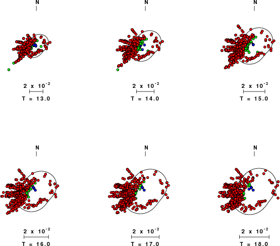
| Focal mechanism sensitivity at the preferred depth. The red color indicates a very good fit to thewavefroms. Each solution is plotted as a vector at a given value of strike and dip with the angle of the vector representing the rake angle, measured, with respect to the upward vertical (N) in the figure. |
The following figure shows the stations used in the grid search for the best focal mechanism to fit the surface-wave spectral amplitudes of the Love and Rayleigh waves.

|
|
|
The surface-wave determined focal mechanism is shown here.
  NODAL PLANES


  STK=     134.99
  DIP=      55.00
 RAKE=      65.00

             OR

  STK=     354.10
  DIP=      42.07
 RAKE=     121.11


DEPTH = 18.0 km

Mw = 5.14
Best Fit 0.8826 - P-T axis plot gives solutions with FIT greater than FIT90
 |
The P-wave first motion data for focal mechanism studies are as follow:
Sta Az Dist First motion
Surface wave analysis was performed using codes from Computer Programs in Seismology, specifically the multiple filter analysis program do_mft and the surface-wave radiation pattern search program srfgrd96.
Digital data were collected, instrument response removed and traces converted
to Z, R an T components. Multiple filter analysis was applied to the Z and T traces to obtain the Rayleigh- and Love-wave spectral amplitudes, respectively.
These were input to the search program which examined all depths between 1 and 25 km
and all possible mechanisms.

|
|
|

|
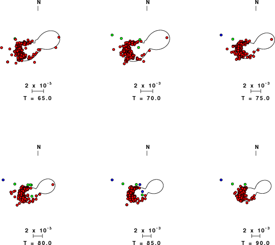
| Pressure-tension axis trends. Since the surface-wave spectra search does not distinguish between P and T axes and since there is a 180 ambiguity in strike, all possible P and T axes are plotted. First motion data and waveforms will be used to select the preferred mechanism. The purpose of this plot is to provide an idea of the possible range of solutions. The P and T-axes for all mechanisms with goodness of fit greater than 0.9 FITMAX (above) are plotted here. |

|
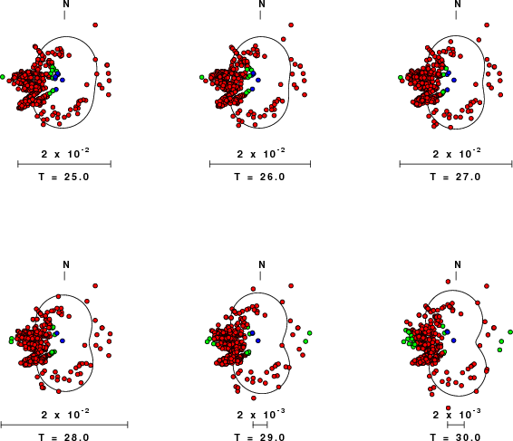
| Focal mechanism sensitivity at the preferred depth. The red color indicates a very good fit to the Love and Rayleigh wave radiation patterns. Each solution is plotted as a vector at a given value of strike and dip with the angle of the vector representing the rake angle, measured, with respect to the upward vertical (N) in the figure. Because of the symmetry of the spectral amplitude rediation patterns, only strikes from 0-180 degrees are sampled. |
The distribution of broadband stations with azimuth and distance is
Listing of broadband stations used
Since the analysis of the surface-wave radiation patterns uses only spectral amplitudes and because the surfave-wave radiation patterns have a 180 degree symmetry, each surface-wave solution consists of four possible focal mechanisms corresponding to the interchange of the P- and T-axes and a roation of the mechanism by 180 degrees. To select one mechanism, P-wave first motion can be used. This was not possible in this case because all the P-wave first motions were emergent ( a feature of the P-wave wave takeoff angle, the station location and the mechanism). The other way to select among the mechanisms is to compute forward synthetics and compare the observed and predicted waveforms.
The fits to the waveforms with the given mechanism are show below:

|
This figure shows the fit to the three components of motion (Z - vertical, R-radial and T - transverse). For each station and component, the observed traces is shown in red and the model predicted trace in blue. The traces represent filtered ground velocity in units of meters/sec (the peak value is printed adjacent to each trace; each pair of traces to plotted to the same scale to emphasize the difference in levels). Both synthetic and observed traces have been filtered using the SAC commands:
hp c 0.02 n 3
lp c 0.10 n 3

|

|
Should the national backbone of the USGS Advanced National Seismic System (ANSS) be implemented with an interstation separation of 300 km, it is very likely that an earthquake such as this would have been recorded at distances on the order of 100-200 km. This means that the closest station would have information on source depth and mechanism that was lacking here.
Dr. Harley Benz, USGS, provided the USGS USNSN digital data. The digital data used in this study were provided by Natural Resources Canada through their AUTODRM site http://www.seismo.nrcan.gc.ca/nwfa/autodrm/autodrm_req_e.php, and IRIS using their BUD interface.
Thanks also to the many seismic network operators whose dedication make this effort possible: University of Alaska, University of Washington, Oregon State University, University of Utah, Montana Bureas of Mines, UC Berkely, Caltech, UC San Diego, Saint L ouis University, Universityof Memphis, Lamont Doehrty Earth Observatory, Boston College, the Iris stations and the Transportable Array of EarthScope.
The CUS used for the waveform synthetic seismograms and for the surface wave eigenfunctions and dispersion is as follows:
MODEL.01
CUS Model with Q from simple gamma values
ISOTROPIC
KGS
FLAT EARTH
1-D
CONSTANT VELOCITY
LINE08
LINE09
LINE10
LINE11
  H(KM) VP(KM/S) VS(KM/S) RHO(GM/CC)   QP   QS  ETAP  ETAS  FREFP  FREFS
  1.0000  5.0000  2.8900  2.5000 0.172E-02 0.387E-02 0.00  0.00  1.00  1.00
  9.0000  6.1000  3.5200  2.7300 0.160E-02 0.363E-02 0.00  0.00  1.00  1.00
 10.0000  6.4000  3.7000  2.8200 0.149E-02 0.336E-02 0.00  0.00  1.00  1.00
 20.0000  6.7000  3.8700  2.9020 0.000E-04 0.000E-04 0.00  0.00  1.00  1.00
  0.0000  8.1500  4.7000  3.3640 0.194E-02 0.431E-02 0.00  0.00  1.00  1.00
Here we tabulate the reasons for not using certain digital data sets
The following stations did not have a valid response files:
DATE=Fri Jun 25 10:28:16 CDT 2010