
2009/11/17 15:30:46 52.080 -131.512 10.0 6.60 British Columbia
USGS Felt map for this earthquake
 USGS/SLU Moment Tensor Solution
 ENS  2009/11/17 15:30:46:7  52.08 -131.51  10.0 6.6 British Columbia

 Stations used:
   AK.BESE AT.CRAG AT.SIT AT.SKAG CN.BBB CN.CBB CN.DLBC CN.EDB
   CN.FNBB CN.HNB CN.HOPB CN.LLLB CN.NLLB CN.PGC CN.PHC CN.PNT
   CN.RUBB CN.SLEB CN.SNB CN.VGZ CN.YOUB UW.LON UW.LTY

 Filtering commands used:
   hp c 0.01 n 3
   lp c 0.025 n 3

 Best Fitting Double Couple
  Mo = 6.61e+25 dyne-cm
  Mw = 6.48
  Z  = 12 km
  Plane   Strike  Dip  Rake
   NP1      173    85   155
   NP2      265    65     5
  Principal Axes:
   Axis    Value   Plunge  Azimuth
    T   6.61e+25     21     126
    N   0.00e+00     65     343
    P  -6.61e+25     14     222

 Moment Tensor: (dyne-cm)
    Component   Value
       Mxx    -1.47e+25
       Mxy    -5.84e+25
       Mxz    -1.26e+24
       Myy     1.03e+25
       Myz     2.80e+25
       Mzz     4.41e+24


                     ####----------
                 ########--------------
              ###########-----------------
             #############-----------------
           ###############-------------------
          ################--------------------
         #################---------------------
        ##################----###---------------
        ##########--------#################-----
       #######-------------####################--
       ###-----------------######################
       #-------------------######################
       --------------------######################
        -------------------#####################
        --------------------####################
         -------------------############   ####
          ------------------############ T ###
           ----   -----------###########   ##
             -- P -----------##############
              -   -----------#############
                 -------------#########
                     ---------#####


 Global CMT Convention Moment Tensor:
      R          T          P
  4.41e+24  -1.26e+24  -2.80e+25
 -1.26e+24  -1.47e+25   5.84e+25
 -2.80e+25   5.84e+25   1.03e+25


Details of the solution is found at

http://www.eas.slu.edu/eqc/eqc_mt/MECH.NA/20091117153046/index.html
|
      STK = 265
      DIP = 65
     RAKE = 5
       MW = 6.48
       HS = 12
The objective of studying this earthquake was to get dispersion for new paths into the new position of the Transportable Array. The waveform solution is not preferred since the earthquake is offshore. The waveform inversion used very long periods, e.g., a bandpass between 0.01 and 0.025 Hz to reduce the influence of the 2-D structure. There are some good waveform fits, although the surface-wave solution is preferred for this earthquake. The surfac-ewave solution has some depth resolution. The surface-wave radiation pattern plots at long periods show the effect of using a velocity model without a proper upper mantle. At shorter periods, the scatter may be due to the fact that a highly attenuating model is assumed, which overcorrects amplitudes at large distances tot he east.
The following compares this source inversion to others
 USGS/SLU Moment Tensor Solution
 ENS  2009/11/17 15:30:46:7  52.08 -131.51  10.0 6.6 British Columbia

 Stations used:
   AK.BESE AT.CRAG AT.SIT AT.SKAG CN.BBB CN.CBB CN.DLBC CN.EDB
   CN.FNBB CN.HNB CN.HOPB CN.LLLB CN.NLLB CN.PGC CN.PHC CN.PNT
   CN.RUBB CN.SLEB CN.SNB CN.VGZ CN.YOUB UW.LON UW.LTY

 Filtering commands used:
   hp c 0.01 n 3
   lp c 0.025 n 3

 Best Fitting Double Couple
  Mo = 6.61e+25 dyne-cm
  Mw = 6.48
  Z  = 12 km
  Plane   Strike  Dip  Rake
   NP1      173    85   155
   NP2      265    65     5
  Principal Axes:
   Axis    Value   Plunge  Azimuth
    T   6.61e+25     21     126
    N   0.00e+00     65     343
    P  -6.61e+25     14     222

 Moment Tensor: (dyne-cm)
    Component   Value
       Mxx    -1.47e+25
       Mxy    -5.84e+25
       Mxz    -1.26e+24
       Myy     1.03e+25
       Myz     2.80e+25
       Mzz     4.41e+24


                     ####----------
                 ########--------------
              ###########-----------------
             #############-----------------
           ###############-------------------
          ################--------------------
         #################---------------------
        ##################----###---------------
        ##########--------#################-----
       #######-------------####################--
       ###-----------------######################
       #-------------------######################
       --------------------######################
        -------------------#####################
        --------------------####################
         -------------------############   ####
          ------------------############ T ###
           ----   -----------###########   ##
             -- P -----------##############
              -   -----------#############
                 -------------#########
                     ---------#####


 Global CMT Convention Moment Tensor:
      R          T          P
  4.41e+24  -1.26e+24  -2.80e+25
 -1.26e+24  -1.47e+25   5.84e+25
 -2.80e+25   5.84e+25   1.03e+25


Details of the solution is found at

http://www.eas.slu.edu/eqc/eqc_mt/MECH.NA/20091117153046/index.html
|
USGS Body-Wave Moment Tensor Solution

 09/11/17 15:30:46.03
 QUEEN CHARLOTTE ISLANDS REGION
 Epicenter:  52.093 -131.419
 MW 6.4

 USGS MOMENT TENSOR SOLUTION
 Depth  14         No. of sta: 81
 Moment Tensor;   Scale 10**18 Nm
   Mrr=-0.41       Mtt=-1.39
   Mpp= 1.79       Mrt= 0.33
   Mrp=-1.15       Mtp= 5.29
  Principal axes:
   T  Val=  5.81  Plg= 6  Azm=126
   N       -0.31      77        4
   P       -5.50      10      217

 Best Double Couple:Mo=5.7*10**18
  NP1:Strike=352 Dip=87 Slip=-168
  NP2:       261     78        -3

               #------
          #######----------
        #########------------
      ###########--------------
    ##############---------------
   ###############----------------
   ###############----------------
  ################-----------------
  #############----################
  ######-----------################
  #----------------################
  ------------------###############
   -----------------##############
   -----------------##########   #
    ----   ---------########## T
      -- P ---------##########
           ----------########
          -----------######
               ------#
|
November 17, 2009, QUEEN CHARLOTTE ISLANDS REGION, MW=6.6

Vala Hjorleifsdottir

CENTROID-MOMENT-TENSOR  SOLUTION
GCMT EVENT:     C200911171530A
DATA: II IU CU IC G  GE
L.P.BODY WAVES:112S, 261C, T= 50
MANTLE WAVES:  106S, 201C, T=125
SURFACE WAVES: 111S, 273C, T= 50
TIMESTAMP:      Q-20091117202117
CENTROID LOCATION:
ORIGIN TIME:      15:30:55.3 0.1
LAT:51.98N 0.00;LON:131.58W 0.01
DEP: 15.5  0.3;TRIANG HDUR:  4.7
MOMENT TENSOR: SCALE 10**25 D-CM
RR= 0.900 0.039; TT=-2.920 0.040
PP= 2.020 0.040; RT= 2.420 0.148
RP=-3.970 0.175; TP= 7.940 0.039
PRINCIPAL AXES:
1.(T) VAL=  8.353;PLG=15;AZM=122
2.(N)       2.072;    63;    359
3.(P)     -10.425;    21;    218
BEST DBLE.COUPLE:M0= 9.39*10**25
NP1: STRIKE=259;DIP=64;SLIP=  -4
NP2: STRIKE=351;DIP=86;SLIP=-154

            ###--------
        ########-----------
      ##########-------------
    ############---------------
   ##############---------------
  ###############----------------
  ############----#############--
 ########---------################
 ####-------------################
 ##---------------################
 ------------------###############
  -----------------##############
  -----------------#########   ##
   -----   --------######### T #
    ---- P ---------########
      --   ---------#########
        ------------#######
            --------###
|
USGS WPhase Moment Tensor Solution

 09/11/17 15:30:46
 QUEEN CHARLOTTE ISLANDS REGION
 Epicenter:  52.079 -131.512
 MW 6.6

 USGS/WPHASE CENTROID MOMENT TENSOR
 09/11/17 15:30:46.00
 Centroid:   52.080 -131.512
 Depth  15         No. of sta: 32
 Moment Tensor;   Scale 10**17 Nm
   Mrr=-0.11       Mtt=-2.01
   Mpp= 2.13       Mrt= 3.94
   Mrp=-5.99       Mtp= 7.28
  Principal axes:
   T  Val=  8.61  Plg=21  Azm=117
   N        2.99      50      358
   P      -11.59      31      221

 Best Double Couple:Mo=1.0*10**19
  NP1:Strike=256 Dip=51 Slip=  -6
  NP2:       351     84      -139

               #------
          ######-----------
        #########------------
      ###########--------------
    ##############---------------
   ########################-------
   #########-------##############-
  #######----------################
  ####-------------################
  ###---------------###############
  #-----------------###############
  ------------------########   ####
   -----------------######## T ###
   -------   --------#######   ###
    ------ P --------############
      ----   --------##########
        -------------########
          -----------######
               ------#
|
USGS Centroid Moment Tensor Solution

 09/11/17 15:30:46.03
 QUEEN CHARLOTTE ISLANDS REGION
 Epicenter:  52.093 -131.419
 MW 6.6

 USGS CENTROID MOMENT TENSOR
 09/11/17 15:31:12.89
 Centroid:   52.547 -131.851
 Depth  22         No. of sta:174
 Moment Tensor;   Scale 10**18 Nm
   Mrr= 0.78       Mtt=-3.11
   Mpp= 2.33       Mrt= 3.78
   Mrp= 0.72       Mtp= 7.59
  Principal axes:
   T  Val=  8.69  Plg=20  Azm=308
   N        0.51      63       87
   P       -9.20      15      212

 Best Double Couple:Mo=8.9*10**18
  NP1:Strike= 81 Dip=87 Slip=  26
  NP2:       350     64       177

               -------
          #######----------
        ###########----------
      ##############-----------
    ###   ###########------------
   #### T ###########-------------
   ####   ############------------
  #####################------------
  #####################---------###
  ####################-############
  #######---------------###########
  ----------------------###########
   ---------------------##########
   ---------------------##########
    -----   ------------#########
      --- P -----------########
        -   -----------######
          ------------#####
               -------
|
The focal mechanism was determined using broadband seismic waveforms. The location of the event and the and stations used for the waveform inversion are shown in the next figure.
|
|
|
|
The program wvfgrd96 was used with good traces observed at short distance to determine the focal mechanism, depth and seismic moment. This technique requires a high quality signal and well determined velocity model for the Green functions. To the extent that these are the quality data, this type of mechanism should be preferred over the radiation pattern technique which requires the separate step of defining the pressure and tension quadrants and the correct strike.
The observed and predicted traces are filtered using the following gsac commands:
hp c 0.01 n 3
lp c 0.025 n 3
The results of this grid search from 0.5 to 19 km depth are as follow:
           DEPTH  STK   DIP  RAKE   MW    FIT
WVFGRD96    0.5    90    75    20   6.16 0.4409
WVFGRD96    1.0    90    70    15   6.18 0.4583
WVFGRD96    2.0    90    70    15   6.21 0.5029
WVFGRD96    3.0    90    70    15   6.23 0.5260
WVFGRD96    4.0    90    70    15   6.25 0.5423
WVFGRD96    5.0    90    70    15   6.26 0.5541
WVFGRD96    6.0    85    75     0   6.26 0.5658
WVFGRD96    7.0    85    75     0   6.28 0.5763
WVFGRD96    8.0    85    75     0   6.29 0.5851
WVFGRD96    9.0    85    75     0   6.30 0.5909
WVFGRD96   10.0    85    75     0   6.31 0.5940
WVFGRD96   11.0    85    80     0   6.31 0.5949
WVFGRD96   12.0    85    80     0   6.32 0.5947
WVFGRD96   13.0    85    80     0   6.33 0.5928
WVFGRD96   14.0    85    80     0   6.33 0.5899
WVFGRD96   15.0    85    80    -5   6.34 0.5860
WVFGRD96   16.0    85    80    -5   6.34 0.5819
WVFGRD96   17.0    85    80   -10   6.35 0.5776
WVFGRD96   18.0    85    80   -10   6.35 0.5731
WVFGRD96   19.0    85    80   -10   6.36 0.5684
WVFGRD96   20.0   265    90     0   6.36 0.5546
WVFGRD96   21.0   270    75    25   6.37 0.5539
WVFGRD96   22.0   270    75    25   6.38 0.5540
WVFGRD96   23.0   270    75    25   6.38 0.5544
WVFGRD96   24.0   270    75    25   6.39 0.5545
WVFGRD96   25.0   270    75    25   6.39 0.5546
WVFGRD96   26.0   270    80    25   6.39 0.5552
WVFGRD96   27.0   270    80    25   6.40 0.5553
WVFGRD96   28.0   270    80    25   6.40 0.5554
WVFGRD96   29.0   270    80    25   6.41 0.5556
The best solution is
WVFGRD96 11.0 85 80 0 6.31 0.5949
The mechanism correspond to the best fit is

|
|
|
The best fit as a function of depth is given in the following figure:

|
|
|
The comparison of the observed and predicted waveforms is given in the next figure. The red traces are the observed and the blue are the predicted. Each observed-predicted componnet is plotted to the same scale and peak amplitudes are indicated by the numbers to the left of each trace. The number in black at the rightr of each predicted traces it the time shift required for maximum correlation between the observed and predicted traces. This time shift is required because the synthetics are not computed at exactly the same distance as the observed and because the velocity model used in the predictions may not be perfect. A positive time shift indicates that the prediction is too fast and should be delayed to match the observed trace (shift to the right in this figure). A negative value indicates that the prediction is too slow. The bandpass filter used in the processing and for the display was
hp c 0.01 n 3
lp c 0.025 n 3

|
|
|

|
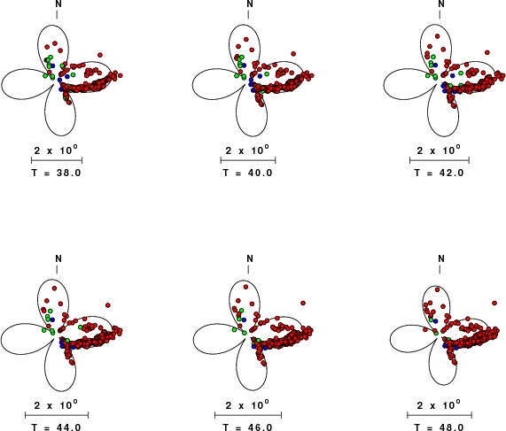
| Focal mechanism sensitivity at the preferred depth. The red color indicates a very good fit to thewavefroms. Each solution is plotted as a vector at a given value of strike and dip with the angle of the vector representing the rake angle, measured, with respect to the upward vertical (N) in the figure. |
The following figure shows the stations used in the grid search for the best focal mechanism to fit the surface-wave spectral amplitudes of the Love and Rayleigh waves.

|
|
|
The surface-wave determined focal mechanism is shown here.
  NODAL PLANES


  STK=     352.88
  DIP=      85.47
 RAKE=     154.92

             OR

  STK=      84.99
  DIP=      65.00
 RAKE=       5.00


DEPTH = 12.0 km

Mw = 6.48
Best Fit 0.8384 - P-T axis plot gives solutions with FIT greater than FIT90
 |
The P-wave first motion data for focal mechanism studies are as follow:
Sta Az Dist First motion
Surface wave analysis was performed using codes from Computer Programs in Seismology, specifically the multiple filter analysis program do_mft and the surface-wave radiation pattern search program srfgrd96.
Digital data were collected, instrument response removed and traces converted
to Z, R an T components. Multiple filter analysis was applied to the Z and T traces to obtain the Rayleigh- and Love-wave spectral amplitudes, respectively.
These were input to the search program which examined all depths between 1 and 25 km
and all possible mechanisms.

|
|
|

|
| Pressure-tension axis trends. Since the surface-wave spectra search does not distinguish between P and T axes and since there is a 180 ambiguity in strike, all possible P and T axes are plotted. First motion data and waveforms will be used to select the preferred mechanism. The purpose of this plot is to provide an idea of the possible range of solutions. The P and T-axes for all mechanisms with goodness of fit greater than 0.9 FITMAX (above) are plotted here. |

|
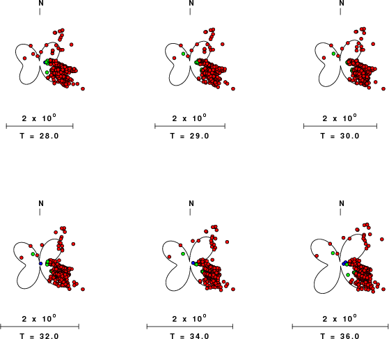
| Focal mechanism sensitivity at the preferred depth. The red color indicates a very good fit to the Love and Rayleigh wave radiation patterns. Each solution is plotted as a vector at a given value of strike and dip with the angle of the vector representing the rake angle, measured, with respect to the upward vertical (N) in the figure. Because of the symmetry of the spectral amplitude rediation patterns, only strikes from 0-180 degrees are sampled. |
The distribution of broadband stations with azimuth and distance is
Listing of broadband stations used
Since the analysis of the surface-wave radiation patterns uses only spectral amplitudes and because the surfave-wave radiation patterns have a 180 degree symmetry, each surface-wave solution consists of four possible focal mechanisms corresponding to the interchange of the P- and T-axes and a roation of the mechanism by 180 degrees. To select one mechanism, P-wave first motion can be used. This was not possible in this case because all the P-wave first motions were emergent ( a feature of the P-wave wave takeoff angle, the station location and the mechanism). The other way to select among the mechanisms is to compute forward synthetics and compare the observed and predicted waveforms.
The fits to the waveforms with the given mechanism are show below:

|
This figure shows the fit to the three components of motion (Z - vertical, R-radial and T - transverse). For each station and component, the observed traces is shown in red and the model predicted trace in blue. The traces represent filtered ground velocity in units of meters/sec (the peak value is printed adjacent to each trace; each pair of traces to plotted to the same scale to emphasize the difference in levels). Both synthetic and observed traces have been filtered using the SAC commands:
hp c 0.01 n 3
lp c 0.025 n 3

|

|
Should the national backbone of the USGS Advanced National Seismic System (ANSS) be implemented with an interstation separation of 300 km, it is very likely that an earthquake such as this would have been recorded at distances on the order of 100-200 km. This means that the closest station would have information on source depth and mechanism that was lacking here.
Dr. Harley Benz, USGS, provided the USGS USNSN digital data. The digital data used in this study were provided by Natural Resources Canada through their AUTODRM site http://www.seismo.nrcan.gc.ca/nwfa/autodrm/autodrm_req_e.php, and IRIS using their BUD interface.
Thanks also to the many seismic network operators whose dedication make this effort possible: University of Alaska, University of Washington, Oregon State University, University of Utah, Montana Bureas of Mines, UC Berkely, Caltech, UC San Diego, Saint L ouis University, Universityof Memphis, Lamont Doehrty Earth Observatory, Boston College, the Iris stations and the Transportable Array of EarthScope.
The used for the waveform synthetic seismograms and for the surface wave eigenfunctions and dispersion is as follows:
MODEL.01
Model after     8 iterations
ISOTROPIC
KGS
FLAT EARTH
1-D
CONSTANT VELOCITY
LINE08
LINE09
LINE10
LINE11
      H(KM)   VP(KM/S)   VS(KM/S) RHO(GM/CC)         QP         QS       ETAP       ETAS      FREFP      FREFS
     1.9000     3.4065     2.0089     2.2150  0.302E-02  0.679E-02   0.00       0.00       1.00       1.00
     6.1000     5.5445     3.2953     2.6089  0.349E-02  0.784E-02   0.00       0.00       1.00       1.00
    13.0000     6.2708     3.7396     2.7812  0.212E-02  0.476E-02   0.00       0.00       1.00       1.00
    19.0000     6.4075     3.7680     2.8223  0.111E-02  0.249E-02   0.00       0.00       1.00       1.00
     0.0000     7.9000     4.6200     3.2760  0.164E-10  0.370E-10   0.00       0.00       1.00       1.00
Here we tabulate the reasons for not using certain digital data sets
The following stations did not have a valid response files:
DATE=Thu Nov 19 08:53:36 CST 2009